Reinforcement learning for collective multi-agent decision making

(1)

Singapore Management University

Institutional Knowledge at Singapore Management University

Dissertations and Theses Collection (Open Access) Dissertations and Theses

12-2018

Reinforcement learning for collective multi-agent

decision making

Duc Thien NGUYEN

Singapore Management University, [email protected]

Follow this and additional works at:https://ink.library.smu.edu.sg/etd_coll

Part of theOS and Networks Commons, and theTheory and Algorithms Commons

Citation

NGUYEN, Duc Thien. Reinforcement learning for collective multi-agent decision making. (2018). Dissertations and Theses Collection (Open Access).

(2)

REINFORCEMENT LEARNING FOR

COLLECTIVE MULTI-AGENT DECISION MAKING

NGUYEN DUC THIEN

SINGAPORE MANAGEMENT UNIVERSITY

2018

(3)

Reinforcement Learning for

Collective Multi-agent Decision Making

Nguyen Duc Thien

Submitted to School of Information Systems in partial fulfillment of the requirements for the Degree of Doctor of Philosophy in Information Systems

Dissertation Committee:

LAUHoong Chuin (Supervisor/Chair) Professor of Information Systems Singapore Management University Akshat KUMAR(Co-Supervisor)

Assistant Professor of Information Systems Singapore Management University

Qin ZHENG

Deputy Department Director

Institute of High Performance Computing, A*STAR Pradeep VARAKANTHAM

Associate Professor

(4)

I hereby declare that this PhD dissertation is my original work and it has been written by me in its entirety.

I have duly acknowledged all the sources of information which have been used in this dissertation.

This PhD dissertation has also not been submitted for any degree in any university previously.

———————————————

Nguyen Duc Thien 6 December 2018

(5)

Reinforcement Learning for

Collective Multi-agent Decision Making

Nguyen Duc Thien

Abstract

In this thesis, we study reinforcement learning algorithms to collectivelyoptimize decentralized policy in a large population of autonomous agents. We notice one of the main bottlenecks in large multi-agent system is the size of the joint trajectory of agents which quickly increases with the number of participating agents. Fur-thermore, thenoiseof actions concurrently executed by different agents in a large system makes it difficult for each agent to estimate the value of its own actions, which is well-known as the multi-agent credit assignment problem. We propose a compact representation for multi-agent systems using the aggregate counts to ad-dress the high complexity of joint state-action and novel reinforcement learning algorithms based on value function decomposition to address the multi-agent credit assignment problem as follows:

1. Collective Representation: In many real-world systems such as urban traffic networks, the joint-reward and environment dynamics depend on only the number of agents (the count) involved in interactions rather than agent identity. We formulate this sub-class of multi-agent systems as a Collective Decentralized Partially Observ-able Markov Decision Process (CDec-POMDP). We show that inCDec-POMDP, the transition counts, which summarize the numbers of agents taking different lo-cal actions and transiting from their current lolo-cal states to new lolo-cal states, are sufficient-statistics for learning/optimizing the decentralized policy. Furthermore, the dimensions of the count variables are not affected by the population size. This

(6)

the counts can be efficiently obtained with multinomial distributions, which provide a faster way to simulate the multi-agent systems and evaluate the planning policy.

2. Collective Multi-agent Reinforcement Learning (MRL): Firstly, to address multi-agent credit assignment problem in_CDec-POMDP, we propose the collective decomposition principle in designing value function approximation and decentral-ized policy update. Under this principle, the decentraldecentral-ized policy of each agent is updated using an individualized value instead of a joint global value. We formu-late a joint update for policies of all agents using the counts, which is much more scalable than independent policy update with joint trajectory. Secondly, based on the collective decomposition principle, we design 2 classes of MRL algorithms for domains with local rewards and for domains with global rewards respectively. i) When the reward is decomposable into local rewards among agents, by exploit-ing exchangeability in CDec-POMDPs we propose a mechanism to estimate the individual value function by using the sampled values of the counts and average individual rewards. We use this count-based individual value function to derive a new actor critic algorithm calledfAfCto learn effective individual policy for agents.

ii) When the reward is non-decomposable, the system performance is evaluated by a single global value function instead of individual value functions. To follow the decomposition principle, we show how to estimate individual contribution value of agents using partial differentials of the joint value function with respect to the state-action counts. This is the basis for us to develop two algorithms calledMCACand CCACto optimize individual policy under non-decomposable reward domains.

Ex-perimentally, we show the superiority of our proposed collective MRL algorithms in various testing domains: a real-world taxi supply-demand matching domain, a police patrolling game and a synthetic robot navigation domain, with population size up to 8000. They converge faster convergence and provide better solutions than other algorithms in the literature, i.e. average-flow based algorithms and standard actor critic algorithm.

(7)

List of Figures

1.1 Example of joint state-action and count table in grid navigation

problem. . . 4

1.2 Multi-agent Reinforcement Learning framework . . . 6

1.3 Multi-agent Reinforcement Learning Classification. . . 8

1.4 Summary of Framework . . . 13

1.5 Chapter dependencies. Included in (·) are chapter numbers with hyperlink. . . 14

2.1 Taxi navigation in zonal map. . . 17

2.2 Robot navigation toward single goal (red location). . . 18

2.3 DBN for T-step reward forCDec-POMDP with external variables . 23 2.4 D-SPAIT model . . . 24

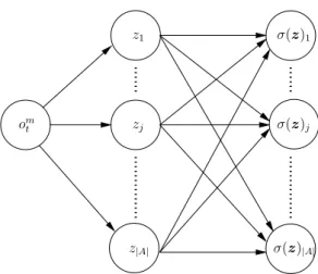
2.5 Simple policy function in which eachzj =✓j⇥omt is a linear trans-formation of the inputom t and the output is the soft-max normaliza-tion. This is known as shadow or no-hidden layer neural network. . 26

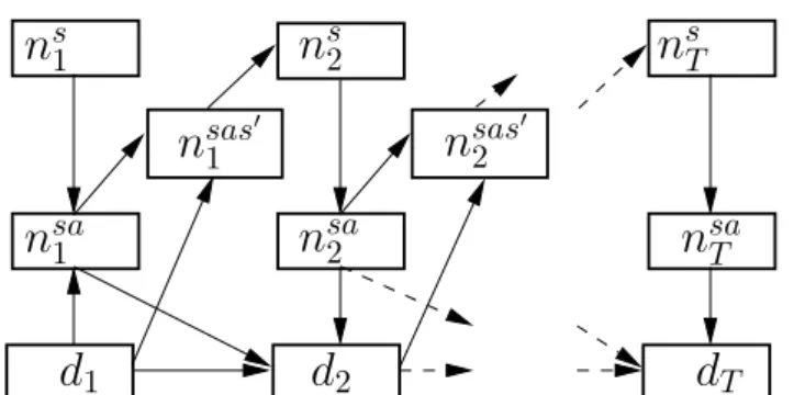
2.6 Generative model of the counts inCDec-POMDP . . . 30 3.1 Example of collective graphical model in a tree model with 4 nodes 42

(14)

4.1 Credit-assignment in multi-agent RL. . . 67 4.2 Credit-assignment in Collective RL. . . 78 4.3 Relation between collective planning and normal MDP planning.

Weliftthe original planning problems with joint state into collective planning problems with collective variables (the count). . . 86

5.1 Example of individual value function estimation from collective sampling. 99

5.2 Solution quality with varying MaxVar in taxi domain . . . 112

5.3 Convergence of average-flow based policy gradient andfAfCoptimizing

static policy on taxi domain. . . 112

5.4 Convergence of different actor-critic variants on the taxi problem. . . 112

5.5 Solution quality with varying population size in grid domain . . . 115

5.6 Convergence of average-flow based policy gradient andfAfCon the grid

navigation problem. . . 115

5.7 Convergence of different actor-critic variants on the grid navigation problem.115

6.1 Solid black lines define 24 patrolling zones of a city district . . . 121

6.2 Convergence of different actor-critic variants on the taxi problem. The

curves forMCACandCCACalmost overlap. . . 133

6.3 Different metrics on the taxi problem with different penalty weightsw. . . 133

6.4 Police patrolling problem. . . 136

6.5 Convergence of different actor-critic variants on the grid patrolling with

varying population sizeN and grid size. . . 137

B.1 Neural Network Architecture for Taxi Problem . . . 176 B.2 Neural Network Architecture for Patrolling Problem . . . 177

(15)

List of Tables

1.1 Summary of contributions in collective multi-agent decision making 12 2.1 Table of Notation . . . 19 A.1 Example of temporal state count for a sectori . . . 170

(16)

Acknowledgements

First and foremost, I thank God for His providence throughout my life, which in-cludes this PhD. I prayed to Him from the beginning to decide on the place to do my PhD, on my research topic, on every submission of my paper. His answers for me have never gone wrong. I worked with the best supervisors in the most interesting research topic to publish the best papers. In addition to all the academic achieve-ments, God also allowed me to travel overseas several times and this made my PhD time more than a joy.

I would like to thank my supervisor, Lau Hoong Chuin, with whom I have been working for almost 7 years since the first day in Singapore. He gave me the opportu-nity to work in various projects with many collaborators. He guided me through this very important part of my career and shaped my character to become an excellent individual and researcher.

I would also like to thank my co-supervisor, Akshat Kumar, who has been work-ing back-to-back with me over many weekend evenwork-ings to rush for submission dead-lines. Akshat taught me how to develop an initial idea into an interesting research direction. We had discussed a lot of interesting concepts during coffee and lunch times and I am sure all of these discussions will be beneficial to my research later. I think by God’s will, I was destined to work with him in my PhD. If I had chosen to come to a different place to do my PhD, he would also be there to help me.

I am also blessed to have many collaborators and good friends during my Ph.D. Amongst them, I would like to thank my supervisor in A?_{STAR, Qin Zheng. Qin}

(17)

has been very supportive in all of the events in my PhD process. I also always remember William Yeoh as my additional advisor, who gave me a lot of useful tips for my PhD. Pradeep Varakantham was always available to help me go through difficult research challenges.

And the final version of my thesis would never be done without the help of my good friends John and Beverly, who have helped to read every of my nearly 200 thesis pages.

Finally, I want to dedicate my PhD to my family, especially my wife. She has been accompanying me in all the sweet and sour moments of my PhD. Without her love and support, I would never have attempted to come to Singapore and finish this PhD.

(18)

(19)

Chapter 1 Introduction

Many real-world problems can be modelled as optimizing actions of autonomous agents over time to maximize some utility or reward functions. Examples include optimizing the movement of autonomous vehicles to serve passengers better, or op-timizing the speed of autonomous vessels to reduce congestion in a port. We can model the decision of each autonomous agent as a decentralized policy function taking input as agent’s local information about the system, such as the congestion level at its current location, and outputs an action, such as the speed or direction to move, for that agent to execute. In this thesis, we study multi-agent reinforce-ment learning (MRL), which is the process to learn decentralized policy function for autonomous agents from empirical reward feedback from environments or sim-ulation engines. The objective of MRL algorithms is to adjust the policy according to the empirical feedback to maximize the expected total rewards over a planning horizon [96, 88, 124]. Reinforcement learning is shown to be efficient methodology to optimize policy in complex domains. Among the most well-studied MRL do-mains are distributed robot systems [5], in which autonomous robots are designed to collaborate with each other to achieve goals, for example to win a robot soccer

(20)

channel network problems, in which a decentralized controller associated to each user needs to independently make decisions about whether to transmit the packet in each specific time slot [42, 145, 85, 84]. In such problems, decentralized controllers have to cooperate to avoid the network conflict and to maximize the total through-put of the network. Other decentralized control problems are studied in power grids [100], traffic light control [32, 142], sensor network control [125, 62], or fire fight-ing teamwork [4]. Recently, with the availability of computfight-ing resources to train artificial neural networks, researchers are able to train neural network policies for multi-agent systems in complex environments such as Atari video games [120] or strategic video game StarCraft [30]. Learning good decentralized policy is shown to enable AI agents to even form their own language as a communicative means to achieve a goal [29, 64].

Although multi-agent reinforcement learning problems have been studied for a long time, the complexity of joint state-action spaces remains a challenge to over-come. In multi-agent systems, each agent could have separate local observations of the environment and independently take action. However their actions will jointly affect each other’s transition and reward. For example, when many vehicles choose to take a specific road, the congestion could slow-down the speed of all vehicles and as a consequence, increase the cost for each vehicle. Because of the interdepen-dence between agents, when optimizing an individual policy, we have to consider all state-actions of the related agents. In this thesis, we use MDP terminology to refer a local “trajectory” as a sequence of local state-actions of a agent and joint “trajectory” as a sequence of joint state-actions of all agents. In multi-agent plan-ning, to estimate the individual value, an agent might need access to jointtrajectory

to know where all other agents are and which actions all other agents take over planning horizon.

In multi-agent systems, the joint state-action space grows exponentially with the number of agents. Mathematically speaking, if local state space of each agent is

(21)

S and its local action space isA, then the size of the joint state-action space ofN

agents(_|S_|_⇥_|A_|)|N|_{. This complexity of the joint space is one of main hurdles to run}

and evaluate contemporary multi-agent reinforcement learning algorithms. Without addressing this scalability, we are a long way from deploying MRL algorithms into real world scenarios consisting of thousands or even millions of agents. This mo-tivates me to develop a compact representation for multi-agent planning problems and subsequently scalable reinforcement learning algorithms for large scale multi-agent systems.

As the basis for scalable multi-agent reinforcement learning algorithms, I pro-pose to use the counts to compactly model a class of multi-agent systems and ef-ficiently optimize individual agent policy in such systems. A count is defined as the number of agents belonging to a particular category, for example to be in a spe-cific local state or location. Counts have been used in many graphical inference problems in machine learning as useful sufficient-statistics [49, 17, 108, 79]. In multi-agent systems, the counts can be used to express the collective behaviors of agents in population and to adjust the collective behaviors according to the feedback from the environment. For instance, the counts used in traffic domains to record the numbers of vehicles coming into each road sector at each time period. By look-ing at the traffic counts, one can reduce the congestion in a sector by adjustlook-ing its heavy incoming flows. In my thesis, to formulate and generalize this count-based decision making concept, I define a model called Collective Decentralized Partially Observable Markov Decision Process (CDec-POMDP) and then develop reinforce-ment learning algorithms to optimize individual policy for multi-agent planning in

(22)

1.1 Collective Decision Making Framework

Before providing further details of our collective planning framework, we give an example of multi-agent domain and compare two representations of the problem. This is followed by the general concept of multi-agent reinforcement learning that we will develop forCDec-POMDPs in this thesis later and a classification of rein-forcement learning methods.

1.1.1 Example of Multi-agent Domain

Goal 0 1 2 3 … … … … left left left up Agent 4 Agent 1 Agent 2 A ge n t 3 (a) A snapshot att= 0. AgentID s0 a0 . . . Agent_1 0 lef t . . . Agent_2 0 lef t . . . Agent_3 0 up . . . . . . . (b) Joint state-action table

hst, atit nsat h0, lef t_it=0 2 h0, upit=0 1 h1, up_it=0 0 . . . . (c) Count table Figure 1.1: Example of joint state-action and count table in grid navigation problem.

We consider robot grid navigation (illustrated in Figure 1.1) as an example of a multi-agent problem. This motivating example is a common testbed for multi-agent reinforcement learning algorithms [132, 66, 76]. In this example, a team of 4 robots try to move in a grid of size3_⇥3toward some goal locations while avoiding conflict

in narrow corridors. A goal could be the representative of a victim in a disaster rescue situation or some object to be picked-up in a transportation task. At each time periodt, a robot in a locationsthas to choose an action as one of 5 movement {lef t, right, up, down, stay}. Consider the snapshot of the grid navigation at time

t = 0. Agents 1,2,3are in location 0, while agent 4is in location 2. From their

local state, agent 1 and 2 take left-turn action while agent3goes up, agent4takes

a left-turn. This can be summarized by the joint state-action Table 1.1b, in which we record the local state, and local action for every agent at every time step. On the

(23)

other hand, we can summarize agent movements by the count Table 1.1c, in which each entrynsa

t (i, j)is the number of agents taking a specific actionjfrom local state

iat timet. As seen in this example, when the number of agents increase, we have to

create new rows to record new agents in a joint state-action Table 1.1b. Meanwhile, the number of entries in the count Table 1.1c is fixed with regard to the number of agents. When the number of agents is significantly larger than the number of local and states and actions, maintaining the count table becomes much more efficient than maintaining the joint state-action table. In MRL, using the counts as input to the decentralized policy and value functions could reduce the input dimensions of those functions in comparison to original joint state-action input. As a result, the counts could improve the scalability and convergence of MRL algorithms.

1.1.2 Multi-agent Reinforcement Learning

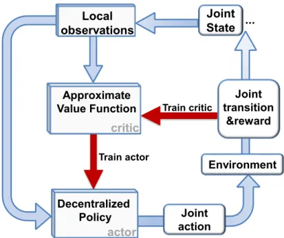
The overview of the MRL framework is illustrated in Figure 1.2. In general, rein-forcement learning is a nature inspired principle to learn action selection function from the reward feedback provided by the environment. In this MRL framework, our goal is to learn a decentralized policy function (called “actor” in the litera-ture) based on the approximation of system’s value (called“critic”in the literature) [117].

At each time step, the decentralized policy function mapslocal observation of an agent to a local action of that agent. Notice that the policy function can be a stochastic function, which produces random actions under an action distribution. After actions are made by agents, they would jointly affect the environment. The result of interaction between joint action and environment is thejoint transitionto the newjoint stateof agents andjoint rewards.

(24)

be the empirical returns (or the total empirical rewards accumulated from the time point when that action is executed). However, due to stochasticity of the problem, empirical return is a random variable with high variance. Furthermore, in multi-agent domains where multiple individual actions are executed at the same time, therawempirical return is too noisy to distinguish roles of concurrent actions. To address this, we a) resort to an approximate value function (“critic”) trained to estimate the empirical return (train critic), and hence resolve the high variance problem of the empirical return, b) propose an efficient policy update to train the policy function (train actor) by the critic.

Train critic Environment Approximate Value Function Decentralized Policy Train actor critic actor Joint action Joint transition &reward Joint State Local observations ...

Figure 1.2: Multi-agent Reinforcement Learning framework

Shared policy

Instead of multiple decentralized policies for different agents, we consider a single decentralized policy function shared by homogeneous agents in the system. In fact, learning ashared (or homogeneous)policy between agents is a common objective in multi-agent reinforcement learning literature [121, 44, 147, 131, 40]. In large scale domains such as movement of animal flocks or a traffic network, a homoge-neous behavior model of individuals is usually assumed [108, 57]. In our research

(25)

problems, by optimizing the shared policy, we can collectivelyshapebehaviors of individuals in favor of system quality. To extend our model to heterogeneous agents, we can generalize shared policy by considering the type of agent as an input feature into the policy function.

Centralized Learning-Decentralized Execution

When an autonomous agent executes its decentralized policy, it only possesses a local view (or partial observation) of the systems. However, inCDec-POMDPs, the dynamicity and the reward of an individual is correlated with others. Local view is sometimes insufficient to learn a decentralized policy. An individual needs to know or estimate behaviors of others to act accordingly [31, 64]. An example in a navigation problem is when an agent knows the intention of another agent is to take a narrow corridor. It could plan to not take that corridor to avoid collision.

To overcome issues of partial observation in policy learning, we would learn the policy by a centralized planner off-line before deploying them into decentralized agents. This centralized planning-decentralized execution paradigm is a common practice in multi-agent reinforcement learning [56]. The centralized planner would reason on either the complete model of the domain [12, 73, 82], or samples of global states generated by a black-box simulator [120]. When neither of these is available, to approximateglobalview, the centralized planner can aggregate local observations from historic data to have a joint view of the system [31]. The global view in the learning phase provides more information for the centralized planner to better estimate value function and refine decentralized policy accordingly. In addition, we can impose the cooperativeness in decentralized policy by the centralized planner. In our collective planning framework, we assume the centralized learner has the access to the joint counts and rewards of the system.

(26)

1.1.3 Reinforcement Learning Classification

Single Agent Multi-agent Collective System

Objective:

Maximize the single agent accumulated reward

Objective:

Maximize the total multi-agent accumulated reward

Objective:

Maximize the total count-based accumulated reward

Environment _Environment _Environment

Collective System State Reward Action Joint State Ind. Rewards

Joint Action State-action counts Transition

counts

Collective rewards

Figure 1.3: Multi-agent Reinforcement Learning Classification.

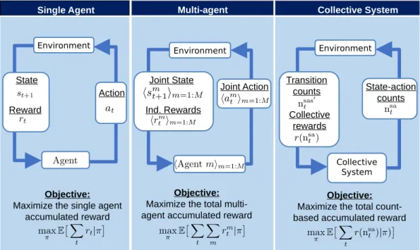
In Figure 1.3, we compare a single agent reinforcement learning system, a multi-agent reinforcement learning system and a collective learning system in a coopera-tive setting. The goal of reinforcement learning algorithm is to optimize the system total rewards through interacting with environment. We want to emphasize the dif-ference in representations of state, reward, action and objective function of the three systems.

In the single agent system, the state, action and reward are singular. The objective in the single agent system is to maximize a single agent expected accumulative reward when the agent interacts with an environment.

The realization of a multi-agent system at timetis represented by samples joint

statehsm

t im=1:M of all agentsm = 1 : M, their actionhamt im=1:M and

correspond-ing joint rewards r(st = hsmt im=1:M,at = hamt im=1:M) depending on the joint

(27)

individual reward as r(st,at) = X m=1:M rm(sm_t , am_t ,st,at). Each rm₍_sm

t , amt ,st,at) represents the reward of agent m receives when it takes

actionam

t in local statesmt and given the joint state-action(st,at).

An objective in a cooperative multi-agent system is to maximize the total expected rewards over planning horizon when multiple agents interact with an environment.

max ⇡ E ⇥ X t r(st,at|⇡ ⇤ = max ⇡ E ⇥ X t X m=1:M rm(sm_t , am_t ,st,at)|⇡ ⇤ .

In the collective planning model, the identity of each agents is marginalized out in collective variables (containing no agent index). The joint statehsmt im=1:M and

actionham

t im=1:M are summarized into the state-action countsnsat . The joint reward

is a function of state-action counts asr(nsa

t ). In some case, the joint reward can be

presented as a sum of individual rewards as

r(nsa_t ) = X i2S,a2A

nsa_t (i, j)r(i, j,nsa_t )

Each rewardr(i, j,nsa

t )represents the average reward of an agent (regardless of

its identity) in stateitaking actionj when the joint state-action counts arensa t . The

joint objective value of the multi-agent reinforcement learning is re-written in the count and average reward variables as

max ⇡ E ⇥ X t r(nsa_t )_|⇡⇤= max ⇡ E ⇥ X t X i2S,a2A nsa_t (i, j)r(i, j,nsa_t )_|⇡⇤.

(28)

large populations, the action count sampling process of collective distribution is generally much cheaper than joint trajectory sampling. More details of collective distribution and sampling process are provided in Chapter 2.

1.2 Summary of Contributions

Our main contributions to the multi-agent collective decision making are two-fold. Firstly, we propose a novel representation for the collective planning problems in

CDec-POMDP model using the count variables. Secondly, based on the new plan-ning representation, we develop count-based reinforcement learplan-ning algorithms to efficiently optimize individual policy for collective planning problems.

1.2.1 Count-based Representation for Collective Planning

Main research challenge: The complexity of multi-agent representation grows when the number of agents in the system increases. This causes a big challenge in managing the state of large population systems for planning purpose. This com-plexity bottleneck is present in our domains of interest, i.e. traffic network and transportation supply-demand matching, where number of agents could vary from 10 to 8000. To address this problem, we propose a compact representation using the count variables.

Technical contributions: We are motivated by the recent advance in collective graphical model (CGM) proposed by Sheldon and Dietterich [108] in showing the counts to be alifted representation of the population. Sheldon and Dietterich [108] show that the counts are sufficient-statistics for inference of collective behaviors. However, CGM is limited in domains where individual policy and transition func-tion of each agent are independent from others. We generalize this nofunc-tion of the

(29)

col-lective representation with the count to multi-agent planning problems by proposing what we term as theCDec-POMDPmodel, in which the transition and reward func-tion of an individual agent depends on the collective behaviour of the populafunc-tion. We show that inCDec-POMDPs, we can marginalize joint trajectory of agents into the count variables. In addition, we show the count variables are sufficient statis-tics for planning in_CDec-POMDP. This means that we can write the global value function inCDec-POMDPs as a function of count variables and we can optimize the objective value ofCDec-POMDPs by changing parameters of the collective dis-tribution of the count variables. The collective disdis-tribution of the count variables provides a fast simulation of the collective system by sampling the counts instead of sampling individual trajectories. This lays the foundation for latter development of efficient planning algorithms using this count representation.

1.2.2 Collective reinforcement learning algorithms

Main research challenge: Due to the complexity of joint trajectory in multi-agent systems, many current multi-agent reinforcement learning (MRL) algorithms are only evaluated in small domains with few agents [58, 120, 30, 31]. We want to exploit the compact representation with the count variables to develop count-based multi-agent reinforcement learning algorithms scalable to large populations. The main research challenge in designing such algorithms is how to estimate thecredit

(as numeric representation of the role) of each individual action to the total reward of the system. The credit provides the local feedback for each agent to update its policy accordingly. In CDec-POMDPs, we have to compute the credit from collective variables instead of the joint trajectories as in the MRL literature.

Technical contributions: Our algorithmic contributions are in development of count-based MRL algorithms using local reward signal and count-based MRL

(30)

algo-based algorithms using the count representation inCDec-POMDPs. We show that the individual value function can be estimated by sampled values of the counts and average rewards. Then we show that we can aggregate policy updates of agents with same state-action into a count-based policy gradient computation. Similar to other fictitious play based algorithms [133], due to the properties inherited from fictitious play, our solution can be also considered as an approximation to the equilibrium in the non-cooperative setting.

When local reward is not available, we train the critic (the value function approx-imator) by the global reward. Then to compute the gradient of the decentralized policy, instead of directly using the global critic, we use its first order Taylor approx-imation. By showing that first order Taylor approximation of the critic is factored amongst agents, we propose an efficient policy gradient computation.

Area Contributions Main techniques

Representation for

col-lective planning Representing collectiveplanning problems us-ing the count C Dec-POMDPs[78, 76]

Collective distribution and sufficient statistics of the count

Collective reinforce-ment learning algo-rithms

Scalable collective factored policy gradient methods [76, 77]

Fictitious play, ex-changeability theorem, Taylor approximation Table 1.1: Summary of contributions in collective multi-agent decision making

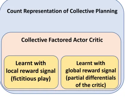
The relation between the components in our framework is demonstrated by the diagram in Figure 1.4. Two new classes of RL algorithms, one with local reward and another with global reward, are proposed based on the factorization form of actor and critic function inCDec-POMDP. The whole framework is developed based on the novel count representation in collective planning.

(31)

Count Representation of Collective Planning

Collective Factored Actor Critic

Learnt with

local reward signal

(fictitious play)

Learnt with

global reward signal

(partial differentials

of the critic)

Figure 1.4: Summary of Framework

1.3 Thesis structure

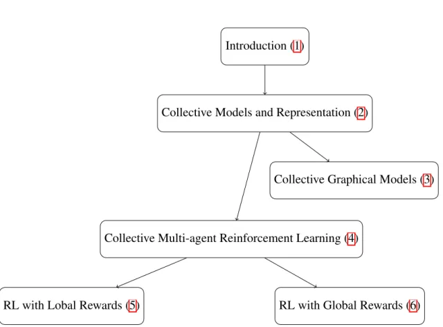
The structure of my thesis is shown in Figure 1.5. After the introduction, in Chap-ter 2, we formulate theCDec-POMDP model and propose the new representation of

CDec-POMDP planning problems using the count variables. In Chapter 3, we intro-duce collective graphical model (CGM) as a predecessor of ourCDec-POMDP. We discuss the connection between collective planning in CDec-POMDP and collec-tive inference in CGM. In Chapter 4, we define colleccollec-tive multi-agent reinforcement learning problems and the related works in multi-agent reinforcement learning liter-ature. We highlight a major challenge in multi-agent reinforcement learning which is thecredit-assignmentfor joint action. To address credit-assignment in collective planning domain, in Chapter 4, we show the factorization of collective policy gradi-ent. The factorization of collective policy gradient is the principle we use to derive collective reinforcement learning algorithms based on local rewards in Chapter 5 and global rewards in Chapter 6. We summarize the main ideas of the thesis and propose future directions in Chapter 7.

(32)

Introduction (1)

Collective Models and Representation (2)

Collective Graphical Models (3)

Collective Multi-agent Reinforcement Learning (4)

RL with Lobal Rewards (5) RL with Global Rewards (6)

Figure 1.5: Chapter dependencies. Included in (·) are chapter numbers with hyper-link.

(33)

Chapter 2 Representation of Collective

Planning

In this chapter, we introduce the collective decentralized (PO)-MDPs (C Dec-POMDP) framework to model multi-agent systems (MAS) where the transition and reward of each individual agent depends on the number (count values) of agents in different local states. First, we show examples of CDec-POMDPs in different multi-agent domains, e.g. taxi supply-demand matching, grid navigation, and pa-trolling (in Section 2.1). Then we formally define the _CDec-POMDP model in Section 2.2. In Section 2.3, we show that count variables are sufficient statistics for planning inCDec-POMDPs. It implies that we can re-write the value functions of aCDec-POMDP with respect to count variables instead of state-action trajectory of agents. By developing the collective distribution of the counts, we propose an effi-cient count sampling procedure to simulate the dynamics of the collective system in Section 2.3.1.

(34)

2.1 Motivation

2.1.1 Taxi Supply Demand problem

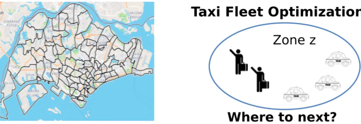
We now present a motivating application for CDec-POMDPs based on the taxi supply demand problem in a zonal city. This is based on the problem introduced in [133]. Figure 2.1 shows the map of Singapore divided into different zones. Our objective is to optimize taxi agent policies to maximize the total profit of the taxi fleet. Such a setting is useful in the case of autonomous taxi fleet operations for revenue maximization. We next describe a taxi agent’s decision making process. At time t, a taxi agent observes its current location in a zone z and also the count

of other taxis in zone z. The agent has two actions: decide to stayin the zone to

look for passengers ormove to another zone (one of 80 other zones). If the agent stays in the current zone, its probability of picking up a passenger is dictated by the ratio between the current demand and the count of other taxis in the zone. If the demand is higher than the number of taxis, then the agent picks up a passenger with a probability close to 1, else the probability is smaller than 1 (based on the ratio of taxis and the current demand). If the agent picks up a passenger, it moves to the passenger’s intended destination. Such transition probabilities can be encoded into the transition function of the CDec-POMDP. The reward an agent gets upon picking a passenger is the total profit of the trip (trip payment minus the fuel cost of moving). If the drive moves to another zone (without a passenger), it incurs the fuel cost for moving.

In this domain, the reward and transition function of each taxi agent is defined by the aggregate count value rather than some specific identity.

(35)

Taxi Fleet Optimization

Zone z

Where to next?

Figure 2.1: Taxi navigation in zonal map.

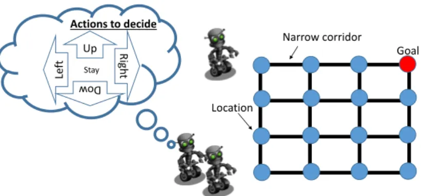
2.1.2 Goal oriented robot navigation

Another domain studied in this thesis is the goal oriented robot navigation. This domain is known as Grid World Problem [118] and has been a testbed for many reinforcement learning algorithms including MAS planning [132, 66]. In this do-main, a team of robots try to move in a grid map toward some goal locations. A goal can be representative of a victim in a disaster rescue scenario or some object to be picked-up in a transportation task. Figure 2.2 shows an example of 3 robots trying to reach a single goal in a4⇥4grid. A robot receives a constant reward whenever

it reaches the goal. Corridors in the grid are narrow, so when there are many robots crossing the same corridor, the transition probability for each robot being able to reach the next location drops dramatically. In other words, the transition function of each robot depends on the number of robots taking the same corridor. In this goal oriented domain, the objective is to maximize the number of times robots reach the goal.

2.1.3 Police Patrolling

We consider the police patrolling problem introduced in [21]. A team of homoge-neous police personnel are stationed in predefined geographic regions to be ready

(36)

Up Ri gh t Le ft Dow Stay Actions to decide Location Narrow corridor Goal

Figure 2.2: Robot navigation toward single goal (red location).

sen to minimize the travel time to the incident location. A police car dispatched to attend an incident would only come back to their locations after a certain of time including traveling and engagement time. When some car leave their stations in critical zones to go to incidents, it is necessary for free police cars in nearby sta-tions to re-allocate to be able to quickly respond to impending emergency. Instead of a centralized police re-allocation, we consider autonomous police agents with a decentralized policy to make decisions on their stations in each decision epoch. An urgent incident is required to be attended within 10 minutes and a non-urgent incident is needed to be attended within 20 minutes. We want to optimize the de-centralized patrolling policy to minimize number of unsatisfied incidents. To model this objective, we consider the penalty -10 whenever the response time requirement of an incident is not met and0otherwise.

Similar to the zonal setting in the taxi domain, we also consider a finite number of locations where police presence can be. However, different from the taxi and robot navigation domains, the number of active agents to make decision is not constant. In other words, only free agents are able to move to new locations. Busy agents would have to come back from all assigned incidents before changing stations. To model this problem with CDec-POMDPs, we extend the local state space of an agent by including the time it would take to become free.

(37)

2.2 Collective

Decentralized

POMDP

(

C

Dec-POMDP) framework

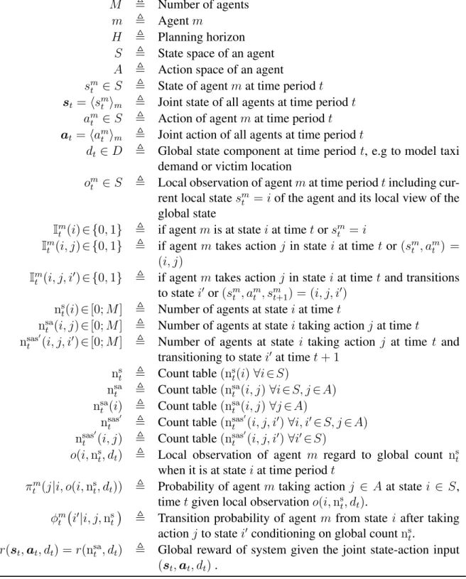
Table 2.1: Table of Notation

M , Number of agents

m , Agentm

H , Planning horizon

S , State space of an agent A , Action space of an agent sm

t 2S , State of agentmat time periodt st =hsmt im , Joint state of all agents at time periodt

am

t 2S , Action of agentmat time periodt at=hamt im , Joint action of all agents at time periodt

dt 2D , Global state component at time periodt, e.g to model taxi

demand or victim location

om

t 2S , Local observation of agentmat time periodtincluding

cur-rent local statesm

t =iof the agent and its local view of the

global state

Im

t (i)2{0,1} , if agentmis at stateiat timetorsmt =i Im

t (i, j)2{0,1} , if agent m takes actionj in state iat time tor(smt , amt ) = (i, j)

Im

t (i, j, i0)2{0,1} , if agentm takes actionj in stateiat timet and transitions

to statei0 or(sm

t , amt , smt+1) = (i, j, i0) ns

t(i)2[0;M] , Number of agents at stateiat timet nsa

t (i, j)2[0;M] , Number of agents at stateitaking actionj at timet nsas0

t (i, j, i0)2[0;M] , Number of agents at state i taking action j at time t and

transitioning to statei0 _{at time}_t_{+ 1}

ns t , Count table(nst(i)8i2S) nsa t , Count table(nsat (i, j)8i2S, j2A) nsa t (i) , Count table(ntsa(i, j)8j2A) nsas0

t , Count table(nsas

0

t (i, j, i0)8i, i02S, j2A) nsas0

t (i, j) , Count table(nsas

0

t (i, j, i0)8i02S)

o(i,ns

t, dt) , Local observation of agent m regard to global count nst

when it is at stateiat time periodt ⇡m

t (j|i, o(i,nst, dt)) , Probability of agent m taking actionj 2 A at statei 2 S,

timetgiven local observationo(i,ns t, dt). m

t i0|i, j,nst , Transition probability of agent m from statei after taking

actionj to statei0 conditioning on global countns t.

(38)

We now formally defineCDec-POMDP as a class of decentralized multi-agent model where agent transition and reward functions are dependent on only the ag-gregate variables. InCDec-POMDP, the identity of an agent is not important and can be marginalized out with the counts. The framework ofCDec-POMDP consists of the following:

• A finite planning horizonH.

• The number of agentsM. An agentmcan be in one of the states in the state

spaceS. We denote a single state asi2S.

• A set of actionAfor each agentm. We denote an individual action asj 2A.

• st,atdenote the joint state and joint action of agents at timet

• We consider a global state component d ₂ D. The joint state space is

⇥M

m=1S⇥D.

• Let(s1:H, a1:H)m= (sm1 , am1 , sm2 . . . , smH, amH)denote the complete state-action

trajectory of an agentm. We denote the state and action of agentmat timet

using random variablessm

t ,amt . Different indicator functionsIt(·)are defined

in Table 2.1. We define the following count given the trajectory of each agent

m₂M: – nsas0 t (i, j, i0) = PM m=1Imt (i, j, i0)8i, i02S, j2A – nsa t (i, j) = PM m=1Imt (i, j) 8i2S, j 2A – ns t(i) = PM m=1Imt (i) 8i2S

As noted in Table 2.1, countnsa

t (i, j)denotes the number of agents in statei

taking action j at time step t; other counts are interpreted analogously. We

denote count tables asns

t = (nst(i)8i2S)andntsa= (nsat (i, j)8i2S, j2A);

tablensas0

(39)

• We assume a general partially observable setting wherein agents can have different observations based on the collective influence of other agents. An agent observes its local state sm

t . In addition, it also observes omt at time t

based on its local statesm

t , the count tablenst, and the global componentdt.

E.g., an agent m in state i at time t can observe the count of other agents

also in state i (=ns

t(i)) or other agents in some neighborhood of the state i

(={ns

t(j)8j 2Nb(i)}). Without loss of generality, we consider the

determin-istic observation functiono(i,ns

t, dt)outputting the same local observation for

all agents in the same statei. To handle stochastic case with different possible

observations in the same state, we can extend the state space to include the observationoi _{which agent receives in a state. The state count is extended to}

record the numbernt(i, oi₎_{of agents in a specific state}_i_{and receiving a same}

observationoi_.

• The local transition function of an agent m is Pl smt+1|stm, amt ,nsat , dt). The

transition function is the same for all the agents. Notice that it is affected by

nsa

t , which depends on the collective behavior of the agent population.

• The transition function of the global componentdisPg(dt+1|dt,nsat ). Notice

that the global component is also affected by state-action count table. • Each agent m has a non-stationary policy ⇡m

t (j|i, o(i,nst, dt)) denoting the

probability of agentmto take actionj given its observation(i, o(i,ns

t, dt))at

timet. We denote the policy over planning horizon of an agentmto be⇡m ₌ (⇡m

1 , . . . ,⇡mH). When agents have the same policy, we denote the common

policy with⇡.

• A reward rt = r(st,at, dt) = r(nsat , dt) is produced for each joint

(40)

• Initial distribution over global component isbg o(d)8d.

In the_CDec-POMDP model, agent identities do not matter; different model compo-nents are only affected by agent’s local state-action, and a statistic of other agents’ states-actions. We define the global component d to model the external variable

besides agents’ local states. In taxi domain, d can be used to model passenger

demands. In patrolling domain, dcan be used to model the victim or incident

oc-currence.

The joint-state transition probability is:

P(st+1, dt+1|st, dt,at) =Pg(dt+1|dt,nsat )· M

Y

m=1

Pl smt+1|smt , amt ,nsat , dt (2.1)

Such an expression conveys that only the statistic nsa

t of the joint state-action, the

global value dand an agent’s local state-action are sufficient to predict the agent’s

next state.

We assume a decentralized and partially observable setting in which each agent receives only a partial observation about the environment. Let the current joint-state be(st, dt)after the last join-action, then the local observation for agentmis given

using the functionot(sm

t , dt,nst). Agents in different states will get different partial

observation about the environment. An agent decides its actionam_{based on its local}

observation as⇡

We consider a general definition of the function r(st, dt,at). In domains like

taxi navigation, this reward can be decomposed into a sum of local rewards of agents

r(st, dt,at) =P_mr(smt ,amt , dt,nsat )wherer(smt ,amt , dt,nsat is the local reward for

individual agent m, which depends on the agent’s local state-action and collective

variables. Given that the reward function is the same for all the agents, we can fur-ther simplify it asPi,jnsat (i, j)r(i, j, dt,nsat ), wherensat (i, j)is the number of agents

(41)

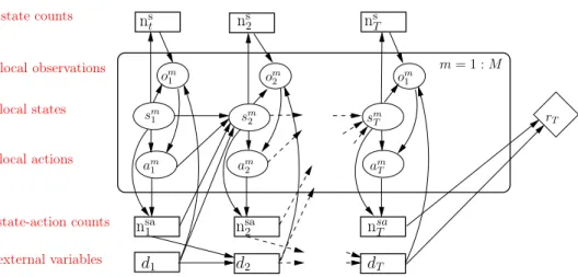
local observations local states local actions state-action counts external variables state counts m= 1 :M om 1 om1 rT sm 1 sm2 am 2 am 1 sm T am T om 2 nsa 2 ns t ns2 dT nsa 1 d2 nsa T ns T d1

Figure 2.3: DBN for T-step reward forCDec-POMDP with external variables for decomposable rewards are studied in Chapter 5 and ones for non-decomposable rewards are studied in Chapter 6 later.

The dynamic Bayesian Network (DBN) for reward collected atTth_{step in}_C

Dec-POMDP is demonstrated with plate notation in Figure 2.3.

Agent type: The above defined model components can also differentiate among agents by using the notion ofagent types, which can be included in the state space. In the extreme case, each agent would be of a different type representing a fairly general multiagent planning problem. However, the main benefit of the model lies in settings when agent types are much smaller than the number of agents.

Policy and value function: We consider a finite-horizon problem with H time

steps. Each agent has a non-stationary reactive policy that takes as input agent’s current stateiand the observationo, and outputs the probability of the next actionj

as⇡m

t (j|i, o). Let⇡=h⇡1, . . . ,⇡Midenote the joint-policy.

InCDec-POMDPs, we consider the goal to find the homogeneous policy ⇡ to

maximize the total rewards over planning horizonH

max ⇡ V(⇡) = H X t=1 E[rt|bo, bgo,⇡] (2.2)

(42)

Average flow approximation

Our model is motivated by the decentralized stochastic planning model (D-SPAIT) for anonymous agents proposed in [131], and the framework of congestion games [68]. In our work, we explicitly model the distribution over countsn(·)of

individuals and use this distribution as the basis for planning. In contrast, the D-SPAIT model is based on the concept of approximating the planning problem using

expected counts of agents. Intuitively, if E[f(n)] denotes the planning objective

over countsn, then D-SPAIT model approximates this objective asf E[n] . Table

2.4a show the computation of such average flow;xst(i)denotes the expected

num-ber of agents in stateiat timetand Figure 2.4b shows DBNs for D-SPAIT model.

Computing policies based on such average flow leads to inaccurate estimation of the true objective function and lower quality policies, as we also demonstrate em-pirically. xs1(i) =M ⇥P(i), 8i2S xstat(i, j) =xst(i)⇥⇡(j|i, xst(i)) 8i2S, j 2A xst+1(i0) = X i,j xstat(i, j) t(i0|i, j, xst(i))8i0 2S

(a) Average approximation of agent flow in D-SPAIT model

x2 xT RT

x1

(b) Deterministic Markov chain for T-step reward Figure 2.4: D-SPAIT model

2.2.1 Policy representation

The benefit of models such as D-SPAIT and CDec-POMDPs lies when the agent population is large, and the agent identity does not affect the reward or the transition function. E.g., in the taxi fleet operation optimization problem discussed earlier

(43)

such aggregate interactions occur. Given a large number of taxis (⇡ 8000), it is

infeasible to compute a unique policy for each taxi. Therefore, similar to the D-SPAIT model, our goal is to compute a homogenous policy⇡for all the agents. As

the policy is dependent on countsnt, it allows for an expressive class of policies.

We define anopen looppolicy as a policy where action selection only depends on the current local state of the agent without any dependence on the count information. In aclosed loop policy, action selection depends on counts also in addition to the agent’s local state. Our proposed model free algorithm developed in the following sections can train both open and closed loop policies, whereas previous average flow based approaches are limited to open loop policy optimization.

Neural network policy

The complexity of closed loop policy would quickly increase when agent observa-tionom

t (i,nst, dt)include not only the count of its current locationnst(i)but

neigh-boring locations{ns

t(j)}j2N(i). In this case, we can consider the policy function to

be neural network⇡m

t :Omt !⌦(A)which takes the input to be possible

observa-tion vectorom

t 2Omt and output the action probability⇡tm(omt ) = h⇡tm(j|omt )ij2A2

⌦(A)with ⌦(A) to be the probability space where P_j₂_A⇡m

t (j|omt ) = 1. To

en-sure the output of policy function to be valid probabilities, we consider the common technique to apply the soft-max normalization for outputz =_hzjij2A

(z)j = P exp(za)

j0₂_Aexp(zj0)

(44)

z1 om t z_|A| zj (z)j (z)1 (z)_|A|

Figure 2.5: Simple policy function in which eachzj =✓j ⇥omt is a linear

transfor-mation of the inputom

t and the output is the soft-max normalization. This is known

as shadow or no-hidden layer neural network.

2.3 Count-based representation of

C

Dec-POMDP

We now establish several basic properties of theCDec-POMDP model. For a fixed population M, let (s1:T,a1:T) = {(s1:T,a1:T)m 8m} denote the state-action

tra-jectories of different agents sampled from the DBN in Figure 2.3. Let n1:T={(nst, nsa

t ,nsas

0

t 8t= 1 :T}be the combined vector of the resulting count tables for each

time stept. We first show that this combined vector is sufficient statistics inC

Dec-POMDP.

Theorem 2.1. Count tablesn1:T are the sufficient statistic for a sample ofM

state-action trajectories from the_CDec-POMDP graphical model in Figure 2.3.

Proof. Let (s1:T,a1:T, d1:T) denote the joint trajectory. The joint-distribution

P(s1:T,a1:T, d1:T;⇡)is defined as:

=bg_o(d) T_Y1 t=1 Pg(dt+1|dt,nsat ) M Y m=1  Y i2S P(i)Imt (i) T_Y1 t=1 Y i,j,i0  ⇡t(j|i, o(i,n_ts, dt))Imt (i,j) Pl(i0|i, j,nsa_t , dt)Imt (i,j,i0)Y i,j ⇡T(j|i, o(i,nsT, dT))I m t (i,j)

(45)

agents. The resulting expressionf(n1:T, d1:T;⇡)depends only on countsn1:T as: f(n1:T, d1:T;⇡) =bg_o(d) T_Y1 t=1 Pg(dt+1|dt,nsat ) Y i2S P(i)ns1(i) T_Y1 t=1 Y i,j,i0  ⇡t(j|i, o(i,n_ts, dt))nsat (i,j) Pl(i0_|i, j,nsa_t , dt)nsast 0(i,j,i0) Y i,j ⇡T(j|i, o(i,nsT, dT))n sa t (i,j) (2.3)

Thus, count tablesn1:T are the sufficient statistic for the population sample as the

joint-probabilityP(s1:T,a1:T, d1:T;⇡)is a function of countsn1:T .

We next define a distribution directly over the count tablesn1:T as below: Theorem 2.2. The distributionP(n1:T, d1:T;⇡)is defined as:1

P(n1:T, d1:T;⇡) =h(n1:T)f(n1:T, d1:T;⇡) (2.4)

wheref(n1:T, d1:T;⇡)is given in (2.3). The functionh(n1:T)counts the total

num-ber of orderedM state-action trajectories with sufficient statistic equal ton, given

as: h(n1:T) = M! Q ins1(i)! T_Y1 t=1 Y i2S  ns t(i)! Q j2Ansat (i, j)! nsa t (i, j)! Q i0₂_Snsast 0(i, j, i0)! ⇥Y i2S  ns T(i)! Q j2AnsaT(i, j)! I[n1:T 2⌦1:T] (2.5) (2.6)

(46)

Set⌦1:T is the set of all allowed consistent count tables as: X i2S ns_t(i) =M 8t;X j2A nsa_t (i, j) = ns_t(i)8j,8t (2.7) X i0 nsas_t 0(i, j, i0) = nsa_t (i, j)₈i₂S, j ₂A,₈t X i,j nsas_t 0(i, j, i0) = ns_t₊₁(i0)₈i0 ₂S,₈t (2.8)

Proof. For any invalid count values n1:T 2/ ⌦1:T, there is no realization of joint

trajectory possessing the invalid count.

We prove the expression forn1:T 2⌦1:T as follows :

P(n1:T, d1:T;⇡) = X hs1:T,a1:Ti⇠n1:T P(_hs1:T,a1:Ti) = X hs1:T,a1:Ti⇠n1:T f(n1:T, d1:T;⇡) (2.9) =h(n1:T)f(n1:T, d1:T;⇡). (2.10)

We prove the expression (2.5) forh(n1:T)by induction:

• WhenT = 1, (2.5) holds ash(n1) = Q M!

i,jnsa1 (i,j) is the total number of

combi-nations to assignM individuals to_|S_|_⇥_|A_|possibilities of state-action. The h(n1)is equivalent to multinomial coefficient of distribution ofM individuals

to|S_|_⇥_|A_|possibilities.

• Assume that (2.5) holds forT. Given a joint trajectorys1:Ta1:T satisfying the

count tablen1:T, the total number of possible joint valuesT+1aT+1satisfying

the count tablenT+1 is

⇣ Y nsa_T(i, j)! Q 0 nsas0(i, j, i0)! ⌘⇣ Y ns T+1(i)! Q i0₂S,j2Ansa (i, j)! ⌘ (2.11)

(47)

Notice that in (2.11), each expression ofi ₂ Sin first term is a multinomial

coefficient of distribution ofnsa

T(i, j)individuals into|S|possibilities of next

statei0 _{to satisfying the count} _nsas0

T (i, j, i0),8i0 ; similarly, each expression

ofi 2Sin second term is a mutinomial coefficient of distribution ofns T+1(i)

individuals in stateiat time stepT + 1into|A|possibilities of actionj.

Multiplying (2.11) with h(n1:T) shows that the expression of h(n1:T+1) as

in (2.5) holds forT + 1, which completes the proof.

One corollary of theorem 2.2 is we can decompose the collective distribution of the count variables as

Corollary 2.1. The collective distribution can be represented by

P(n1:T, d1:T;⇡) =P(nsaT |nsT, dT)bgo(d)P(ns1) Y t=1:T 1 Pg(dt+1|dt,nsat )P(nsat |nst, dt)P(nsas 0 t |nsat , dt)I[n1:T 2⌦1:T], in which P(ns 1) = M! Q ins1(i)! Y i2S bo(i)n s 1(i) (2.12) P(nsa_t |ns_t, dt) = Y i2S ⇣ _ns t(i)! Q j2Ansat (i, j)! Y j2A ⇡t(j|i, o(i, dt,nst))n sa t (i,j) ⌘ (2.13) P(nsas_t 0_|nsa_t , dt) = Y i2S,j2A ⇣ _nsa t (i, j)! Q i0₂_Snsast 0(i, j, i0)! Y i0₂S Pl(i0_|i, j,nsa_t , dt)nsast 0(i,j,i0) ⌘ (2.14) The Bayesian graphical model of the collective distribution is shown in Figure 2.6.

(48)

d2

d1

d

T

n

s₁

n

sa₁

n

s₂

n

sa₂

n

s_T

n

sa_T

n

sas₁ 0

n

sas₂ 0

Figure 2.6: Generative model of the counts inCDec-POMDP

2.3.1 Count Sampling Process

Originally, as a summary of joint trajectory, the count variables are obtained by aggregating values of individual variables. However, sampling individual values would be computationally expensive in large populations. Fortunately, the collec-tive distribution of the counts shown in corollary 2.1 can provide us a way todirectly

sample the count values instead of aggregating the individual variables. As genera-tive model of the count is a Bayesian network (in Figure 2.6), we can generate the values of the counts by forward sampling from state-count to action count and then transition count.

Algorithm 1 provides the pseudo code to generate the count samples forHtime

periods. The state count in the first period is sampled by the multinomial distribu-tion with a populadistribu-tion size to be M and probabilities to be the initial distribution bo (line 2). At each time period t, we sample action counts for agents at each

lo-cal state iby multinomial distribution with population size ns

t(i) and probabilities

⇡t(j|i, o(i,ns

t, dt)) (line 5). Analogously, to simulate the effect of the joint action

counts into the environment, we can sample the transition count for agents tak-ing actionj from the local stateiby multinomial distribution with population size

nsa

(49)

Algorithm 1:Collective Sampling Algorithm

1 AlgorithmC-SA M P L I N G()

2 Samplingns₁ _⇠Mul(M, bo)

3 Samplingd1⇠bgo

4 fort 1toHdo

5 Sampling state-action counts:nsa_t (i,•)⇠Mul(ns_t(i),⇡t(•|i, o(i, dt,nst))),

8i₂S

6 Sampling transition counts:

nsas0

t (i, j,•)⇠Mul(nsat (i, j), Pl(•|i, j,nsat , dt)),8i2S, j 2A

7 Sampling external variables:dt+1⇠Pg(•|dt,nsat )

8 Aggregate: ns t+1(i0) = P i,jnsas 0 t (i, j, i0),8i0 2S 9 returnn1:H

2.3.2 Joint-Value Function

We next show that the joint-value for a given policy ⇡ also depends on the count

vector n. Thus, making counts as the sufficient statistic for planning in C

Dec-POMDPs.

Theorem 2.3. The joint-value function of a policy⇡over horizonHgiven by the

ex-pectation of total rewards,V(⇡) =PH_T₌₁E[rT], can be computed by the expectation

over counts as:

X n2⌦1:H P(n1:H, d1:H;⇡) _XH T=1 rT(nsaT, dT) (2.15)

Proof. Let sT andaT represent the joint-state and joint-action of all the agents at

the time stepT;ns

T andnsaT represent the count vectors corresponding to(sT,aT).

The immediate reward received for this joint-state and action is r(sT,aT, dT) =

rT(nsaT , dT).

(50)

E[rT(⇡)]

= X

(s1:T 1,a1:T 1,d1:T 1),sT

P(s1:T 1,a1:T 1, dT 1)P(sT|sT 1,aT 1)rT(sT, dT;⇡)

(2.16)

usingCDec-POMDP distribution, we have:

= X

(s1:T,a1:T,d1:T)⇠n1:T,d1:T

f(n1:T, d1:T)rT(nsaT , dT) (2.17)

Notice that in the above expression, the expected immediate reward at time stepT

only depends on the counts nsa

T that arise from the joint state and action(sT,aT).

Similar to equations (2.9) and (2.10), instead of summing over all the joint state-action trajectories(s1:T,a1:T, d1:T), we can sum over the space of all possible counts

vectorsn1:T multiplied by the total number of joint trajectories satisfying the

corre-sponding counts vectorn1:T, which results in the following expression: E[rT(⇡)] = X d1:T X n1:T2⌦1:T h(n1:T)f(n1:T, d1:T)  X nsa T⇠nsT P(nsa_T |nsa_T , dT)rT(nsaT, dT) (2.18) Using the above expression, the value function can be computed as:

V(⇡) = H X T=1 E[rT] = H X T=1 X n1:T2⌦1:T,d1:T P(n1:T, d1:T)rT(nsaT, dT) (2.19)

Our goal in CDec-POMDP is to compute the policy ⇡ that maximizes (2.15).

Notice that the set of all the allowed counts⌦1:H is combinatorially large, making

the exact policy evaluation infeasible. Therefore, our approach would be to use a sampling based approach that can evaluate, and also optimize the policy⇡.

(51)

joint state-action countsQ⇡

t(st,at, dt) =Q⇡t(nsat , dt) =

PH

T=tE[rT|nsat , dt]:

Theorem 2.4. The joint state-action value function in_CDec-POMDP is defined by

Q⇡_t(nsa_t , dt) =rt(nsa_t , dt) + X nsas0 t ,nsat+12⌦t+1,dt+1 P(dt+1|nsat , dt) ⇥P(nsas_t 0_|nsa_t , dt)P(nsa_t₊₁_|ns_t₊₁ _⇠nsas_t 0, dt+1;⇡)Q⇡t+1(nsat+1, dt+1) (2.20) in which P(nsa t |nst, dt), P(nsas 0

t |nsat , dt) are defined in corollary 2.1. ⌦t+1 is the

subset of consistency constraints(2.7)linking counts for timetandt+1

Proof. We start by the general dynamic programming equation for MDP [117] with noticert =r(st,at, dt) = r(nsat , dt) Q⇡_t(st,at, dt) =r(nsat , dt) + X st+1,at+1,dt+1 P(st+1, dt+1|st,at, dt)P(st+1,at|st+1, dt+1;⇡)Q⇡t+1(st+1,at+1, dt+1) (2.21) Using similar arguments as in the proof of theorem 2.2, we can aggre-gate similar hst,at,st+1i by hnst,nsat ,nsas

0

t i and consider induction hypothesis

Q⇡ t+1(st+1,at+1, dt+1) =Q⇡t+1(nsat+1, dt+1) Q⇡_t(st,at, dt) = rt(nsat , dt) + X nsas0 t ,nsat+12⌦t+1,dt+1 P(dt+1|nsat , dt) ⇥P(nsas0 t |nsat , dt)P(nsat+1|nst+1 ⇠nsas 0 t , dt+1;⇡)Qt⇡+1(nsat+1, dt+1)

The right hand side of above equation is an expression over counts, which defines

Q⇡

(52)

2.4 Related works

2.4.1 Count-based models

In many multi-agent systems (MAS), the transition and reward of each individual in the population is affected by aggregate values rather than the identity of agents. Among the most well-studied domains is the class of congestion games [68, 80], in which the pay-off function of each agent is defined only by the number of other agents traveling on the same edges. The congestion game has a wide range of applications in modeling the delay cost of road traffic flow [112, 136], and latency in package routing in communication network such as the Internet [95]. Besides the aggregate-variable pay-off function, the state transition of each agent also can be modeled as a function of aggregate values [131, 97, 113] . For example, in routing problem, after executing a moving action, high congestion level (or high number of agents presenting) in the same area could reduce the probability of agent arriving the next zone [132]. Apart from the congestion game, aggregate-variable transition functions are also defined in action graph games[47], in which the transition of an agent depends on the aggregate value of its neighbors. In the disease control domain, Robbel et al. [97] modelled the vulnerability to of a geological zone by the number of its disease-infected neighbors . In riot control, Sonu et al. [113] studied the protest intensity depending on the number of protestors and the number of police troops presenting in a location.

Our application domains in goal-oriented robot navigation and taxi supply-demand matching were studied previously by Varakantham et al. [131, 133]. We consider our domain setting similar to the ones in [133, 131]. However, our count variables provide the exact representation of_CDec-POMDP while the average flow is an approximate representation.

(53)

2.4.2 Mean-field game theory and average flow estimations

To deal with planning problems in large population of agents, researchers in the current literature have been trying to estimate the planning problems with tractable representation. One amongst these well-studied directions is the mean-field estima-tion of populaestima-tion [146, 140] in continuous state-acestima-tion space. Rooted in mean-field theory in physics to estimate the distribution of individual particles in systems, the mean-field methods quantify population behavior by the density function of dis-tribution of agents over continuous spaces. It assumes each individual in a large population has a very small impact on the global distribution. As a result, the dy-namic of the population can be represented in the form of a differential equation of continuous (flow of agents) variables. Examples of mean-field systems include fish school, ant colonies or flocks of birds [15] in nature or swarm robotics in AI [11, 103]. In domain of discrete state-action space, Varakantham et al. [133, 131] explored a similar idea with mean-field by estimating average flows of agents into each discrete state-action in a finite Markov Decision Process (MDP). By using the average flow estimation, multi-agent planning problems are re-formulated as network flow problems with non-linear flow splitting constraints induced from the MDP transition function. Based on the average flow variables, Varakantham et al. [133] proposed a individual value function estimation, which facilitated fictitious play computation of the policy. In addition, as the average flow MDP has Varakan-tham et al. [131] showed that the average flow MDP problem can be modeled and solved by a mathematics programming. Average flow and mean-field methods are empirically shown to achieve good results in some domains. However, it is worth noting that these methods provide only an estimation of the original problem, and this estimation can incur a high approximation error when the transition function is highly non-linear.

Reinforcement learning for collective multi-agent decision making

Singapore Management University

Institutional Knowledge at Singapore Management University

Reinforcement learning for collective multi-agent

decision making

Duc Thien NGUYEN

REINFORCEMENT LEARNING FOR

COLLECTIVE MULTI-AGENT DECISION MAKING

NGUYEN DUC THIEN

SINGAPORE MANAGEMENT UNIVERSITY

2018

Reinforcement Learning for

Collective Multi-agent Decision Making

Nguyen Duc Thien

———————————————

Reinforcement Learning for

Collective Multi-agent Decision Making

Nguyen Duc Thien

Abstract

Contents

List of Figures

List of Tables

Acknowledgements

Chapter 1

Introduction

1.1 Collective Decision Making Framework

1.1.1 Example of Multi-agent Domain

1.1.2 Multi-agent Reinforcement Learning

1.1.3 Reinforcement Learning Classification

1.2 Summary of Contributions

1.2.1 Count-based Representation for Collective Planning

1.2.2 Collective reinforcement learning algorithms

Count Representation of Collective Planning

Collective Factored Actor Critic

Learnt with

local reward signal

(fictitious play)

Learnt with

global reward signal

(partial differentials

of the critic)

1.3 Thesis structure

Chapter 2

Representation of Collective

Planning

2.1 Motivation

2.1.1 Taxi Supply Demand problem

Taxi Fleet Optimization

Zone z

Where to next?

2.1.2 Goal oriented robot navigation

2.1.3 Police Patrolling

2.2 Collective

Decentralized

POMDP

(

C

Dec-POMDP) framework

2.2.1 Policy representation

2.3 Count-based representation of

C

Dec-POMDP

d2

d1

d

n

n

n

n

n

n

n

n

2.3.1 Count Sampling Process

2.3.2 Joint-Value Function

2.4 Related works

2.4.1 Count-based models

2.4.2 Mean-field game theory and average flow estimations