optimization models
Isabel Eguía1, María Araceli Garín2, and Aitziber Unzueta1 1Dpto. Matemática Aplicada,
Universidad del País Vasco, UPV/EHU Bilbao (Bizkaia), Spain
e-mail: [email protected] e-mail: [email protected] 2Dpto. de Economía Aplicada III,
Universidad del País Vasco, UPV/EHU Bilbao (Bizkaia), Spain
e-mail: [email protected]
Abstract
Stochastic optimization problems of practical applications lead, in general, to some large models. The size of those models is linked to the number of scenarios that defines the sce-nario tree. This number of scesce-narios can be so large that decomposition strategies are required for problem solving in reasonable computing time. Methodologies such as Branch-and-Fix Coordination and Lagrangean Relaxation make use of these decomposition approaches, where independent scenario clusters are given. In this work, we present a technique to generate clus-ter submodel structures from the decomposition of a general two-stage stochastic mixed integer optimization model. Scenario cluster submodels are generated from the original stochastic prob-lem by combining the compact and splitting variable representations in some of the variables related to the nodes that belong to the first stage. We consider a two-stage stochastic capacity expansion problem as illustrative example where several decompositions are provided.
Keywords:Stochastic Optimization, Scenario Cluster Partitioning, C++ code , MPS format.
∗This research has been partially supported by the projects MTM2015-65317-P from the Spanish Ministry of Econ-omy and Competitiveness, PPG17/32 and GIU 17/011 from the University of the Basque Country, UPV/EHU, and Grupo de Investigación IT-928-16 from the Basque Government.
1
Introduction
Stochastic optimization problems of practical applications lead, in general, to some large models. The size of those models is linked to the number of scenarios that define the scenario tree. This number of scenarios can be so large that decomposition strategies are required for problem solving in reasonable time. For theory, methodologies and algorithms in relation with stochastic optimization see [4, 6, 25, 29]and [30], among many others.
Most of the optimization problems require integer variables, mainly 0-1 variables besides con-tinuous ones. The advantage of a mixed 0-1 approach is that it provides a general framework for modeling a large variety of problems.
The traditional aim in this type of problems is to solve the Deterministic Equivalent Model (for short, DEM), which usually is a mixed 0-1 problem with a special structure. Exact decomposition algorithms for solving the DEM have been studied for different types of problems, see [21, 32]. Some of them combining with a Branch-and-Bound method to deal with the integer variables, see our work in [8, 10, 12] as well as [26], among others.
Some approaches for multistage problems where appear most promising to use the information about the separability of the problem are presented in [24, 27, 28], just for naming a few works. Specifically, see in [8, 9, 10, 11, 12, 15, 31, 32, 35], among others, some decomposition approaches that consider scenario clustering or grouping for solving large-scale multistage stochastic mixed integer problems. The so-named Branch-and-Fix Coordination (BFC) methodology is used in the decomposition approaches presented in [8, 10, 12, 15] to generate independent scenario clusters such that multiplicity of any scenario is not allowed among the clusters. Moreover, Lagrangean Decomposition (for short, LD) [13, 14, 16, 17, 18] can be used as part of a solution methodology. In a first step, consists of relaxing the so-called nonanticipativity constraints (for short, NAC) for some of the stages. Then, scenario cluster submodels are generated from the original stochastic problem by dualizing the NAC related to the nodes that belong to the stages up to the break one. Subgradient Method (SM)[19, 20], Volume Algorithm (VA) [3], Lagrangean Progressive Hedging Algorithm (LPHA) [30, 13] and Dynamic Constrained Cutting Plane (DCCP) algorithm [22] can then be used in the Lagrangean multipliers updating scheme, while solving multi-stage mixed 0-1 submodels based on scenario cluster decomposition, see [14]. The proximal bundle method presented in [23] can be also used as a Lagrangean multipliers updating scheme. In all these cases it is proved that the tightness of the bounds can be increased “by grouping together scenarios”.
In general, for any multi-stage stochastic problem withT stages and|Ω|scenarios, the infor-mation about until what stage the scenario submodels have common inforinfor-mation, is saved in the scenario tree. See in [2], for the details of the general procedure of scenario cluster partitioning, based in the break stage concept in case of general multi-stage problems.
In the case of two-stage problems the simpler structure of the scenario tree allows to use an easy procedure to decompose the full model. About scenario cluster partitioning in two-stage models, see [13]. In this paper, a scenario clustering is presented where the number of clusters can be chosen from the set of divisors of the number of scenarios, |Ω|. Now, we propose the generalization of this procedure such that be possible to choose the number of clusters as any value from the set
The rest of the paper is organized as follows. Section 2 deals with the main concepts and related notation of a two-stage optimization model. Section 3 presents the scenario clustering scheme. Section 4 presents an example as illustrative case. Section 5 introduces the files required for the decomposition. Section 6 reports the results of the decomposition procedure over the illustrative case; and, Section 7 concludes.
Some Appendices present the detail of some MPS files, a part of the C++ code, and some other information.
2
Two-stage model
Let us consider the following two-stage stochastic mixed 0-1 model incompactrepresentation:
(MIP): zMIP =min a1x1+b1y1+Eψ[aω2x2ω+bω2yω2]
s.t. A x1 y1 ≤h1 T x1 y1 +Wω xω2 yω2 ≤hω2, ∀ω∈Ω y1,y ω 2 ≥0, ∀ω∈Ω x1,x ω 2 ∈ {0,1}, ∀ω∈Ω (1)
wherea1andb1are known vectors of the objective function coefficients for the 0-1 and continuous
variables in the first stagex1andy1, respectively,h1is the right hand side vector for the first stage
constraints, andAis the known matrix of coefficients for the first stage constraints. For each scenario ω,hω2 is the right hand side vector for the second stage constraints; andaω2 andbω2 are the objective function coefficients for the second stage variables 0-1 and continuous, xω2 and yω2 respectively. Furthermore,TandWω are the technology matrices, this second under scenarioω, forω∈Ω, where Ωis the set of scenarios to consider. Piecing together the stochastic components of the problem, we have a vector ψω = (aω2,b ω 2,h ω 2,W ω), with ω ∈Ω. Finally, E
ψ represents the mathematical expectation with respect toψ over the set of scenariosΩ.
All this information can be represented as a tree in which each path from the root to the leaf corresponds to a specific scenarioω. In addition, each node of the tree can be associated with a group of scenariosgwhereG denotes the set of scenario groups (i.e. nodes in the underlying scenario tree),
andGt, the subset of scenario groups that belong to staget∈T, such thatG =∪t∈TGt andΩgis
the set of the scenarios related to groupg. Finally,T denotes the set of stages and in our particular case,|T|=2.
Sometimes it can be useful to work with scenarios instead of with nodes or groups, for example if you want to split the set of scenarios into different subsets. Ωgdenotes the set of scenarios that belong to groupg, forg∈G.
1 t=1 (x1,y1) |Ω|+1 3 2 t=2 (x12,y12) (x22,y22) (x|2Ω|,y |Ω| 2 ) ω =|Ω| ω=2 ω=1 1 t=1 (x11,y11) (x21,y21) (x|1Ω|,y |Ω| 1 ) 1 1 2 3 |Ω|+1 t=2 (x12,y12) (x22,y22) (x|2Ω|,y|2Ω|) ω=|Ω| ω=2 ω=1
Compact representation Splitting variable representation
Figure 1: Scenarios tree
The left part of Figure 1 corresponds to the compact representation of the problem in which there is only one copy of each first stage variable. In this part, the concept of scenario group is used to represent the nonanticipativity constrains implicitly. It corresponds to the representation given in model (1).
The right part of Figure 1 corresponds to the splitting variable representation of the problem, given in model (4), in which there is a replica of each first stage variable for each scenario. In this way, in the first stage we must impose the nonanticipativity constrains in the variablesxω1 andyω1 for the scenariosωthat belong the same groupΩg,g∈G1={1}, i.e., for all scenarios,ω∈Ω.
Following the nonanticipativity principle stated in [34] and restated in [30] see also [4], among many others, both scenarios should have the same value for the related variables with the same index up to the given stage. The conditions called Non-Anticipativity Constrains (NAC) establish in particular in the two-stage models that the decisions of the first stage must be independent of the scenario in which they occur and, therefore, be the same under the different scenarios. So that
xω = xω′, ∀ω,ω ′∈Ω ,ω6=ω ′ (2) yω = yω′, ∀ω,ω ′∈Ω ,ω6=ω ′ (3)
Similar the NAC must be satisfied by all the coefficients vectors and matrices of the first stage
(aω1,b ω 1,h ω 1,A ω ,T ω).
(MIP): zMIP = min∑ω∈Ω∑2t=1wω(atω xωt +btωytω) s.t. Aω xω1 yω1 ≤hω1, ∀ω∈Ω Tω xω1 yω1 +Wω xω2 yω2 ≤hω2, ∀ω∈Ω xω=xω′, ∀ω,ω ′∈Ω ,ω 6=ω ′ yω=yω′, ∀ω,ω ′∈Ω ,ω 6=ω ′ yω≥0, ∀ω∈Ω xω∈ {0,1}, ∀ω∈Ω (4)
wherewω is the likelihood attributed to each scenarioω.
Throughout the following sections we will describe a procedure to generate the cluster submodel structures from the descomposition of a general full model.
3
Scenario Cluster Partitioning
In order to combine the compact and the splitting variable representation, we propose a cluster scenario partition of the full model, being a scenario cluster a set of scenarios where the NAC constrains are implicitly considered.
In general, for any multi-stage stochastic problem withT stages and|Ω|scenarios, the informa-tion about until what stage the scenario submodels have common informainforma-tion, and when the NAC must be explicit, is saved in the subsetsGt andΩg, g∈Gt,t∈T, i.e., in the scenario tree. Then, a general procedure of scenario cluster partitioning based in the break stage concept is developped. See [10], [12] and [2], for the definition of this concept and related topics.
In the case of two-stage problems the simple structure of the scenario tree allows to use an easy procedure to decompose the whole model. See [13] a scenario cluster partitioning of two-stage models,where the number of clusters can be chosen from the set of divisors of the number of scenarios,|Ω|. In this work , we propose the generalization of this procedure such that is possible to choose the number of clusters as any value from the setC ={1,2,· · ·,|Ω|}.
Definition 1 Thescenario tree matrix, ST ∈M|Ω|x|G|, is a matrix where the corresponding value for
the pair(ω,g)gives the related stage t,such that,
ST(ω,g) =
t, i f ω ∈Ωg, g∈Gt
0, otherwise
(5)
Notice that the scenario tree matrix reproduces the structure given by the scenario tree. This matrix can be built using the setsΩgandGt, i.e., the scenario tree, but these sets can be also generated
from the matrix. For each staget∈T, the sets of scenario groups in such stage,Gt, can be identified as the column of the position(ω,g)for which the corresponding element in the scenario tree matrix
is equal tot; thenGt={g∈G :∃ω∈Ω:ST(ω,g) =t}. See also that the set of scenarios related to
groupgisΩg={ω∈Ω:ST(ω,g)6=0}.
Then, given the choice of the number of clusters,C=|C|, we will decompose the scenario tree
into a subset of scenario clusters subtrees, each one for each scenario cluster in the set denoted as
C ={1, ...,C}.
LetΩc denote the set of scenarios that belongs to cluster c, wherec∈C and∑C
c=1|Ωc|=|Ω|. Notice thatΩcT Ωc′ =/0,c ,c ′=1 , . . . ,C:c6=c ′andΩ=∪C c=1Ωc.
Let alsoGc⊂G denote the set of scenario groups for cluster c, such thatΩ
g∩Ωc6= /0 means thatg∈Gc, and letGc
t =Gt∩Gcdenote the set of scenario groups for clusterc∈C in staget∈T. Definition 2 Thescenario cluster models are those that result from the relaxation of some of the NAC in model (1).
In the same way that for the full scenario tree, for a cluster subtree, we can reproduce its structure by using a matrix.
Definition 3 Thecluster tree matrixassociated with a partition into C clusters, CT ∈MCx|G|, is a
matrix where the corresponding value for the pair(c,g)gives the related stage t,such that,
CT(c,g) = t, i f g∈G c t 0, otherwise (6)
Once decided the number of clustersC, the corresponding cluster partition is obtained, and its struc-ture is defined by the related cluster tree matrix. In two-stage models, and from the definition of cluster submodels, a way to create each partition is to consider the integer division of the number of scenarios over the desired number of clusters, |ΩC|, and if this quotient is not equal to zero, distribute the remaining scenarios among the different clusters, starting by the first cluster and continuing un-til the remaining scenarios are finished. The implementation in C++ of this procedure is shown in Appendix B. See also the example of scenario cluster partitioning in Section 6.
Notice thatGc
t =Gt∩Gc, is the set of scenario groups for cluster c∈C, in staget∈T. The subsetsGcandG
t and, consequentlyGtccan be obtained from the cluster tree matrix defined above. For each clusterc∈C (i.e.,c−row in the CT matrix), the set of scenario groupsGccan be obtained as the set of columns in the cluster tree matrix with a nonzero element, i.e.,Gc={g∈G :∃c∈C :
CT(c,g) =t}.
Then, we can decompose the whole model into splitting variable representation between the cluster models and add explicitly the nonanticipativity constraints into the diferent clusters. Notice also that we consider compact representation into each cluster model.
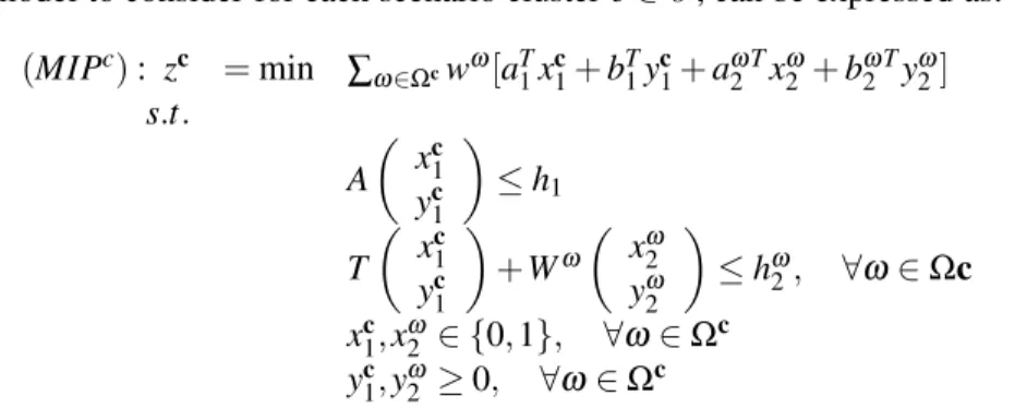
The submodel to consider for each scenario clusterc∈C, can be expressed as: (MIPc): zc =min ∑ω∈Ωcwω[aT1xc1+bT1yc1+aωT2 xω2 +bωT2 yω2] s.t. A xc1 yc1 ≤h1 T xc1 yc1 +Wω xω2 yω2 ≤hω2, ∀ω∈Ωc xc1,x ω 2 ∈ {0,1}, ∀ω∈Ω c yc1,y ω 2 ≥0, ∀ω∈Ω c (7)
The following figure illustrates the cluster generation proposed depending on whether the num-ber of scenarios of the problem is even or odd.
t=1 1 c=2 |Ω|+1 |Ω| 2 +3 |Ω| 2 +2 1 c=1 |Ω| 2 +1 3 2 t=2 ω=|Ω| ω=|Ω2|+2 ω=|Ω2|+1 ω=|Ω2| ω=2 ω=1 t=1 1 c=2 |Ω|+1 ⌊|Ω|2⌋+4 ⌊|Ω|2⌋+3 1 c=1 ⌊|Ω|2⌋+2 ⌊|Ω|2⌋+1 3 2 t=2 ω=|Ω| ω=⌊|Ω2|⌋+3 ω=⌊|Ω2|⌋+2 ω=⌊|Ω2|⌋+1 ω=⌊|Ω2|⌋ ω=2 ω=1 ⌊|Ω2|⌋=|Ω2| ⌊|Ω2|⌋ 6=|Ω2|
4
Illustrative example
Consider the following two-stage stochastic capacity expansion problem based on the multistage one presented in [1].
The mixed 0-1 model has the following form: min
∑
i∈I (a1i x1i+e1iy1i) +∑
ω∈Ω wω∑
i∈I (aω2ixω2i+eω2iyω2i) s.t.y1i≤M1ix1i ∀i∈I yω2i≤M2ωi x2ωi ∀i∈I, ∀ω∈ Ω∑
i∈I y1i≥d1∑
i∈I (yω2i+y1i)≥d2ω ∀ω ∈ Ω x1i, x ω 2i∈ {0,1}, y1i,y ω 2i∈R+ ∀i∈I, ∀ω∈ Ω (8)whereI denotes the set of resources or technology types.The goal is to determine a schedule of
tim-ing and level of capacity acquisitions of setI to satisfy the demandsd1andd2ω , while minimizing
the expected discounted cost over the set of scenarios along the time horizon. The decision continu-ous variablesy1iandyω2i denote the capacity expansion of resource typei∈I andx1iandxω2i denote the 0-1 decision variables for the corresponding capacity expansion decision fori∈I. Without loss of generality, we assume zero initial capacities. Moreover,a1i andaω2i are the discounted fixedand for resourcei∈I;e1iandeω
2iare the variable investment cost for resourcei∈I andM1i andM2ωi are the variable upper bound on the capacity additions fori∈I.
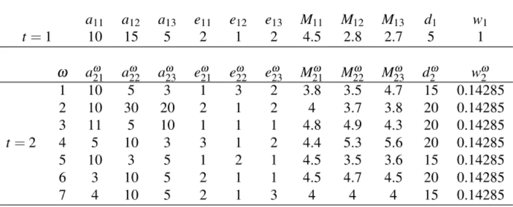
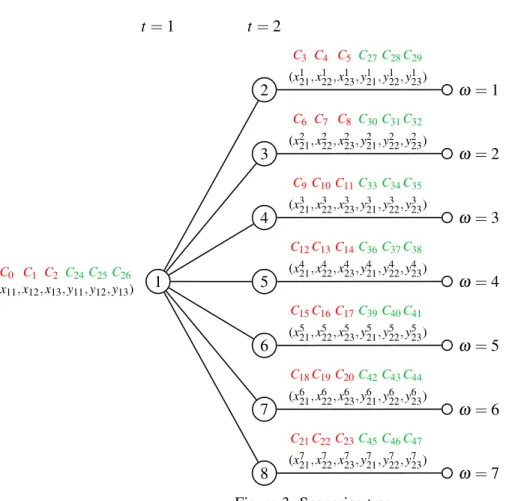
Table 1 gives the problem data. It is assumed that the uncertain parameters given in Table 1 refer to the scenario tree structure depicted in Figure 3, being the solution valuez=78.841185.
Notice that the number of scenarios in the example is seven and there are three 0-1 variables and three continuous variables in each scenario group and each stage, all of them with the same probability. Moreover, the order of these variables in the input data is exactly the given in Figure 3, as it can be seen in the MPS format of Appendix A.
Table 1: Illustrative example parameters
a11 a12 a13 e11 e12 e13 M11 M12 M13 d1 w1 t=1 10 15 5 2 1 2 4.5 2.8 2.7 5 1 ω aω21 aω22 aω23 eω21 eω22 eω23 M21ω M22ω M23ω d2ω wω2 t=2 1 10 5 3 1 3 2 3.8 3.5 4.7 15 0.14285 2 10 30 20 2 1 2 4 3.7 3.8 20 0.14285 3 11 5 10 1 1 1 4.8 4.9 4.3 20 0.14285 4 5 10 3 3 1 2 4.4 5.3 5.6 20 0.14285 5 10 3 5 1 2 1 4.5 3.5 3.6 15 0.14285 6 3 10 5 2 1 1 4.5 4.7 4.5 20 0.14285 7 4 10 5 2 1 3 4 4 4 15 0.14285
1 t=1 8 7 6 5 4 3 2 t=2 (x11,x12,x13,y11,y12,y13) C0 C1 C2 C24C25C26 (x121,x122,x123,y121,y 1 22,y123) C3 C4 C5 C27C28C29 (x221,x222,x223,y221,y 2 22,y223) C6 C7 C8 C30C31C32 (x321,x322,x323,y321,y 3 22,y323) C9C10C11C33C34C35 (x421,x422,x423,y421,y 4 22,y 4 23) C12C13C14C36C37C38 (x521,x522,x523,y521,y 5 22,y 5 23) C15C16C17C39C40C41 (x621,x622,x623,y621,y 6 22,y623) C18C19C20C42C43C44 (x721,x722,x723,y721,y 7 22,y723) C21C22C23C45C46C47 ω=7 ω=6 ω=5 ω=4 ω=3 ω=2 ω=1
Figure 3: Scenarios tree
min 10x11+15x12+5x13+1.4285x 1 21+0.71425x 1 22+0.42855x 1 23 + 1.4285x 2 21+4.2855x 2 22+2.857x 2 23+1.57135x 3 21+0.71425x 3 22+1.4285x 3 23 + 0.71425x 4 21+1.4285x 4 22+0.42855x 4 23+1.4285x 5 21+0.42855x 5 22+0.71425x 5 23 + 0.42855x 6 21+1.4285x 6 22+0.71425x 6 23+0.5714x 7 21+1.4285x 7 22+0.71425x 7 23 + 2y11+y12+2y13+0.14285y 1 21+0.42855y 1 22+0.2857y 1 23 + 0.2857y 2 21+0.14285y 2 22+0.2857y 2 23+0.14285y 3 21+0.14285y 3 22+0.14285y 3 23 + 0.42855y 4 21+0.14285y 4 22+0.2857y 4 23+0.14285y 5 21+0.2857y 5 22+0.14285y 5 23 + 0.2857y 6 21+0.14285y 6 22+0.14285y 6 23+0.2857y 7 21+0.14285y 7 22+0.42855y 7 23 s.t. −4.5x11+y11≤0 −2.8x12+y12≤0 −2.7x13+y13≤0 −3.8x 1 21+y121≤0 −3.5x 1 22+y122≤0 −4.7x 1 23+y123≤0 −4x221+y221≤0 −3.7x 2 22+y222≤0 −3.8x 2 23+y223≤0 −4.8x 3 21+y321≤0 −4.9x 3 22+y322≤0 −4.3x 3 23+y323≤0 −4.4x 4 21+y421≤0 −5.3x 4 22+y422≤0 −5.6x 4 23+y423≤0 −4.5x 5 21+y521≤0 −3.5x 5 22+y522≤0 −3.6x 5 23+y523≤0 −4.5x 6 21+y621≤0 −4.7x 6 22+y622≤0 −4.5x 6 23+y623≤0 −4x721+y721≤0 −4x722+y722≤0 −4x723+y723≤0 y11+y12+y13≥5 y11+y12+y13+y211 +y122+y123≥15 y11+y12+y13+y212 +y222+y223≥20 y11+y12+y13+y213 +y322+y323≥20 y11+y12+y13+y214 +y422+y423≥20 y11+y12+y13+y215 +y522+y523≥15 y11+y12+y13+y216 +y622+y623≥20 y11+y12+y13+y217 +y722+y723≥15 y1i,y ω 2i≥0, ∀i∈I, ∀ω∈Ω x1i,x ω 2i∈ {0,1}, ∀i∈I, ∀ω∈Ω (9)
5
Basic requeriments
Given a two-stage stochastic mixed integer optimization model, and for the aim of obtaining the sce-nario cluster partition, some additional information is required. This information has been organized in two files:
1. A file (in this case called total.mps, see Appendix A) with the two-stage model in compact representation (4) in MPS format.
2. An input file so-calledinputData.datwith the following information:
• C, number of clusters in which the model is going to be descomposed
• Number of scenario groups in each stage
• nxt,t=1,2, number of 0-1 variables by stage (number of 0-1 variables in any scenario
group)
• nyt,t=1,2, number of continuous variables by stage (number of continuous variables
in any scenario group)
• wω,ω ∈Ω, vector of likelihood for scenarios. If all scenarios have the same probability of occurrence, 0 value appears in the corresponding line.
• γ, parameter that takes value 1 if the order of variables is the expected one, and 0 in other case. The order of variables is the expected one when first all the 0-1 variables, and then, all the continuous one are stored. Moreover, in each variable type, they are ordered by stage and in each stage, ordered by scenario.
• oxi,i=1,· · ·,nx;oyi, i=1,· · ·,ny, position of the variables such they are included in
the model, being nxandnythe number of 0-1 and continuous variables respectively. If the original order of variables in the MPS file is the expected one, 0 value appears in this line. 1 4 1 2 4 8 3 2 2 2 2 2 2 2 0 0 0 0 5 2 2 2 2 16 23 17 24 18 25 19 26 20 27 21 28 22 29 0 8 1 9 2 10 3 11 4 12 5 13 6 14 7 15 inputData.dat
The first data in file inputData.dat corresponds to the number of clusters, C, that in this ex-ample is 2. There are|G1|=1, |G2|=|Ω|=7 scenario groups. Then, in both stages, there are
(nx1,ny1)=(nx2,ny2) =(3,3)variables in each scenario group. So, in the first stage there are 3 binary
variables and 3 continuos ones, while in the second stage there are 21 binary and 21 continuous, respectively.
The likelihood for each scenario is the same, equal to 17, and then, the corresponding data in the file is a 0.
Finally, the 0-1 variables in the model (total.mps file) appear in the following order: 0 1 2 6 7 8, ...
While the order for the continuos ones, is: 3 4 5 9 10 11, ...
This means, that these variables (0-1 and continuos) appear mixed at each stage and scenario group: x11,x12,x13,y11,y12,y13,x 1 21,x 1 22,x 1 23,y 1 21,y 1 22,y 1 23, ...,x 7 21,x 7 22,x 7 23,y 7 21,y 7 22,y 7 23
while the expected or required order in the model, needed to start the decomposition is, first all the binaries and after, all the continuos:
x11,x12,x13,x 1 21,x 1 22,x 1 23, ...,x 7 21,x 7 22,x 7 23 y11,y12,y13,y 1 21,y 1 22,y 1 23, ...,y 7 21,y 7 22,y 7 23
In this way, they are saved in the model after the first steps of the procedure, see below.
6
Example. Scenario Cluster Partitioning
The scenario tree matrixST(ω,g)corresponding to the illustrative example is given in (10).
ST(ω,g) = 1 2 0 0 0 0 0 0 1 0 2 0 0 0 0 0 1 0 0 2 0 0 0 0 1 0 0 0 2 0 0 0 1 0 0 0 0 2 0 0 1 0 0 0 0 0 2 0 1 0 0 0 0 0 0 2 (10)
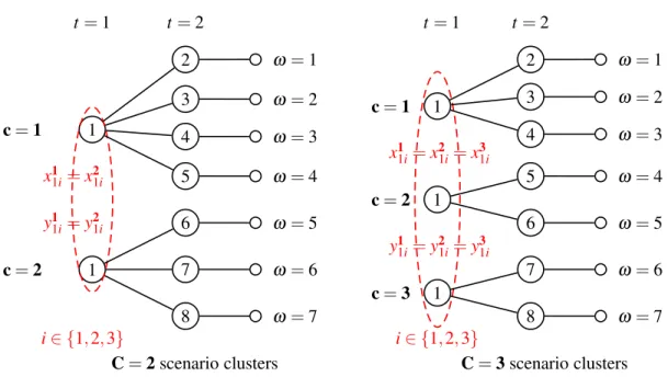
In the ilustrative example depicted in Figure 3, firstly, we are going to consider in a first partition thatC=2. As |ΩC| =7
2 =3.5, the integer division is equal to 3, and, then, the rest is equal to 1. As
output of the procedure, we obtain that the first cluster is given by the scenarios amongminwc[0] =1 andmaxwc[0] =4 and the second one, by the scenarios amongminwc[1] =5 andmaxwc[1] =7. See the left part of Figure 4.
Then, the cluster tree matrix associated to this partition is given in (11).
CT(c,g) = 1 2 2 2 2 0 0 0 1 0 0 0 0 2 2 2 (11)
In this case, the set of scenarios areΩ1={1
,2,3,4} for cluster c=1 and Ω 2={5
,6,7} for
t=1 y11i=y21i=y31i i∈ {1,2,3} x11i=x21i=x31i 1 c=3 8 7 1 c=2 6 5 1 c=1 4 3 2 t=2 ω=7 ω=6 ω=5 ω=4 ω=3 ω=2 ω=1 t=1 1 c=2 8 y11i=y21i i∈ {1,2,3} x11i=x21i 7 6 1 c=1 5 4 3 2 t=2 ω=7 ω=6 ω=5 ω=4 ω=3 ω=2 ω=1
C=2scenario clusters C=3scenario clusters
Figure 4: Scenario cluster partitioning
x11i=x21i, ∀i∈I (12)
y11i=y21i, ∀i∈I (13)
min 10x111+15x112+5x113+1.4285x 1 21+0.71425x 1 22+0.42855x 1 23 + 1.4285x 2 21+4.2855x 2 22+2.857x 2 23+1.57135x 3 21+0.71425x 3 22+1.4285x 3 23 + 0.71425x 4 21+1.4285x 4 22+0.42855x 4 23+2y111+y112+2y113 + 0.14285y 1 21+0.42855y 1 22+0.2857y 1 23+0.2857y 2 21+0.14285y 2 22+0.2857y 2 23 + 0.14285y 3 21+0.14285y 3 22+0.14285y 3 23+0.42855y 4 21+0.14285y 4 22+0.2857y 4 23 s.t. −4.5x 1 11+y111≤0 −2.8x 1 12+y112≤0 −2.7x 1 13+y113≤0 −3.8x 1 21+y121≤0 −3.5x 1 22+y122≤0 −4.7x 1 23+y123≤0 −4x221+y221≤0 −3.7x 2 22+y222≤0 −3.8x 2 23+y223≤0 −4.8x 3 21+y321≤0 −4.9x 3 22+y322≤0 −4.3x 3 23+y323≤0 −4.4x 4 21+y421≤0 −5.3x 4 22+y422≤0 −5.6x 4 23+y423≤0 y111+y112+y113≥5 y111+y112+y113+y121+y122+y123≥15 y111+y112+y113+y221+y222+y223≥20 y111+y112+y113+y321+y322+y323≥20 y111+y112+y113+y421+y422+y423≥20 y11i,y ω 2i≥0, ∀i∈I,ω∈Ω 1 x11i,x ω 2i∈ {0,1}, ∀i∈I,ω∈Ω 1 (14)
Notice that this cluster has 15 integer variables and 15 continuous variables, 20 constraints, 57 nonzero elements and the value of the objective function iszMIP=49.5845.
min 10x211+15x212+5x213+1.4285x 5 21+0.42855x 5 22+0.71425x 5 23 + 0.42855x 6 21+1.4285x 6 22+0.71425x 6 23+0.5714x 7 21+1.4285x 7 22+0.71425x 7 23 + 2y211+y212+2y213+0.14285y 5 21+0.2857y 5 22+0.14285y 5 23 + 0.2857y 6 21+0.14285y 6 22+0.14285y 6 23+0.2857y 7 21+0.14285y 7 22+0.42855y 7 23 s.t. −4.5x 2 11+y211≤0 −2.8x 2 12+y212≤0 −2.7x 2 13+y213≤0 −4.5x 5 21+y521≤0 −3.5x 5 22+y522≤0 −3.6x 5 23+y523≤0 −4.5x 6 21+y621≤0 −4.7x 6 22+y622≤0 −4.5x 6 23+y623≤0 −4x721+y721≤0 −4x722+y722≤0 −4x723+y723≤0 y211+y212+y213≥5 y211+y212+y213+y521+y522+y523≥15 y211+y212+y213+y621+y622+y623≥20 y211+y212+y213+y721+y722+y723≥15 y21i,y ω 2i≥0, ∀i∈I,ω∈Ω 2 x21i,x ω 2i∈ {0,1}, ∀i∈I,ω∈Ω 2 (15)
The clusterc=2 has 12 integer variables and 12 continuous variables, 16 constraints, 45 nonzero elements and the value of the objective function for this cluster iszMIP=24.3994.
If we choose,C=3, i.e., a partition into three clusters, folowing the same procedure (|ΩC| =73 =
2.33, and rest equal to 1) we obtain that the first cluster is given by the scenarios amongminwc[0] =1
andmaxwc[0] =3, the second one by the scenarios amongminwc[1] =4 andmaxwc[1] =5, and the third one by the scenarios amongminwc[2] =6 andmaxwc[2] =7. Then, the corresponded cluster tree matrix will be,
CT(c,g) = 1 2 2 2 0 0 0 0 1 0 0 0 2 2 0 0 1 0 0 0 0 0 2 2 (16)
In this partition, the set of scenarios areΩ1={1
,2,3}for clusterc=1,Ω 2={4
,5}for cluster
c=2 andΩ3={6
,7}for clusterc=3. The related cluster models are linked by the NAC forg=1
that can be expressed
x11i=x21i=x31i, ∀i∈I (17)
The clusterc=1 has 12 integer variables and 12 continuous variables, 16 constraints, 45 nonzero elements and the value of the objective function iszMIP=38.799. The clusterc=2 has 9 integer
variables and 9 continuous variables, 12 constraints, 33 nonzero elements and the value of the objec-tive function iszMIP=17.3995 and the clusterc=3 has 9 integer variables and 9 continuous
vari-ables, 12 constraints, 33 nonzero elements and the value of the objective function iszMIP=16.971.
7
Conclusions
In this brief note we have presented a general scenario cluster partitioning procedure for two-stage models. To generate the new structure and representation of the two-stage model some information is required, like the whole model in compact representation andmpsformat, the number of clusters in which the model is going to be decomposed, the number of scenarios, the number and the order of the variables (binary and continuous) at each stage and scenario group and the likelihood of each scenario.
The use of this procedure embedded in a cluster based Lagrangian decomposition scheme, and for a choice of a small number of clusters, will allow to obtain strong (lower) bounds to the solution value of the original two-stage stochastic problem.
Appendix A
Illustrative stochastic example in MPS format
The model corresponding to the example presented in (9) can be represented with MPS format as follows: NAME BLANK 2 ROWS N OBJROW 4 L R0000000 L R0000001 6 L R0000002 L R0000003 8 L R0000004 L R0000005 10 L R0000006 L R0000007 12 L R0000008 L R0000009 14 L R0000010 L R0000011 16 L R0000012 L R0000013 18 L R0000014 L R0000015 20 L R0000016 L R0000017 22 L R0000018 L R0000019 24 L R0000020
L R0000021 26 L R0000022 L R0000023 28 G R0000024 G R0000025 30 G R0000026 G R0000027 32 G R0000028 G R0000029 34 G R0000030 G R0000031 36 COLUMNS C0000000 OBJROW 1 0 . R0000000 −4.5 38 C0000001 OBJROW 1 5 . R0000001 −2.8 C0000002 OBJROW 5 . R0000002 −2.7 40 C0000003 OBJROW 2 . R0000000 1 . C0000003 R0000024 1 . R0000025 1 . 42 C0000003 R0000026 1 . R0000027 1 . C0000003 R0000028 1 . R0000029 1 . 44 C0000003 R0000030 1 . R0000031 1 . C0000004 OBJROW 1 . R0000001 1 . 46 C0000004 R0000024 1 . R0000025 1 . C0000004 R0000026 1 . R0000027 1 . 48 C0000004 R0000028 1 . R0000029 1 . C0000004 R0000030 1 . R0000031 1 . 50 C0000005 OBJROW 2 . R0000002 1 . C0000005 R0000024 1 . R0000025 1 . 52 C0000005 R0000026 1 . R0000027 1 . C0000005 R0000028 1 . R0000029 1 . 54 C0000005 R0000030 1 . R0000031 1 . C0000006 OBJROW 1 . 4 2 8 5 R0000003 −3.8 56 C0000007 OBJROW 0 . 7 1 4 2 5 R0000004 −3.5 C0000008 OBJROW 0 . 4 2 8 5 5 R0000005 −4.7 58 C0000009 OBJROW 0 . 1 4 2 8 5 R0000003 1 . C0000009 R0000025 1 . 60 C0000010 OBJROW 0 . 4 2 8 5 5 R0000004 1 . C0000010 R0000025 1 . 62 C0000011 OBJROW 0 . 2 8 5 7 R0000005 1 . C0000011 R0000025 1 . 64 C0000012 OBJROW 1 . 4 2 8 5 R0000006 −4. C0000013 OBJROW 4 . 2 8 5 5 R0000007 −3.7 66 C0000014 OBJROW 2 . 8 5 7 R0000008 −3.8 C0000015 OBJROW 0 . 2 8 5 7 R0000006 1 . 68 C0000015 R0000026 1 . C0000016 OBJROW 0 . 1 4 2 8 5 R0000007 1 . 70 C0000016 R0000026 1 . C0000017 OBJROW 0 . 2 8 5 7 R0000008 1 . 72 C0000017 R0000026 1 . C0000018 OBJROW 1 . 5 7 1 3 5 R0000009 −4.8 74 C0000019 OBJROW 0 . 7 1 4 2 5 R0000010 −4.9 C0000020 OBJROW 1 . 4 2 8 5 R0000011 −4.3 76 C0000021 OBJROW 0 . 1 4 2 8 5 R0000009 1 . C0000021 R0000027 1 . 78 C0000022 OBJROW 0 . 1 4 2 8 5 R0000010 1 .
C0000022 R0000027 1 . 80 C0000023 OBJROW 0 . 1 4 2 8 5 R0000011 1 . C0000023 R0000027 1 . 82 C0000024 OBJROW 0 . 7 1 4 2 5 R0000012 −4.4 C0000025 OBJROW 1 . 4 2 8 5 R0000013 −5.3 84 C0000026 OBJROW 0 . 4 2 8 5 5 R0000014 −5.6 C0000027 OBJROW 0 . 4 2 8 5 5 R0000012 1 . 86 C0000027 R0000028 1 . C0000028 OBJROW 0 . 1 4 2 8 5 R0000013 1 . 88 C0000028 R0000028 1 . C0000029 OBJROW 0 . 2 8 5 7 R0000014 1 . 90 C0000029 R0000028 1 . C0000030 OBJROW 1 . 4 2 8 5 R0000015 −4.5 92 C0000031 OBJROW 0 . 4 2 8 5 5 R0000016 −3.5 C0000032 OBJROW 0 . 7 1 4 2 5 R0000017 −3.6 94 C0000033 OBJROW 0 . 1 4 2 8 5 R0000015 1 . C0000033 R0000029 1 . 96 C0000034 OBJROW 0 . 2 8 5 7 R0000016 1 . C0000034 R0000029 1 . 98 C0000035 OBJROW 0 . 1 4 2 8 5 R0000017 1 . C0000035 R0000029 1 . 100 C0000036 OBJROW 0 . 4 2 8 5 5 R0000018 −4.5 C0000037 OBJROW 1 . 4 2 8 5 R0000019 −4.7 102 C0000038 OBJROW 0 . 7 1 4 2 5 R0000020 −4.5 C0000039 OBJROW 0 . 2 8 5 7 R0000018 1 . 104 C0000039 R0000030 1 . C0000040 OBJROW 0 . 1 4 2 8 5 R0000019 1 . 106 C0000040 R0000030 1 . C0000041 OBJROW 0 . 1 4 2 8 5 R0000020 1 . 108 C0000041 R0000030 1 . C0000042 OBJROW 0 . 5 7 1 4 R0000021 −4. 110 C0000043 OBJROW 1 . 4 2 8 5 R0000022 −4. C0000044 OBJROW 0 . 7 1 4 2 5 R0000023 −4. 112 C0000045 OBJROW 0 . 2 8 5 7 R0000021 1 . C0000045 R0000031 1 . 114 C0000046 OBJROW 0 . 1 4 2 8 5 R0000022 1 . C0000046 R0000031 1 . 116 C0000047 OBJROW 0 . 4 2 8 5 5 R0000023 1 . C0000047 R0000031 1 . 118 RHS RHS R0000024 5 . R0000025 1 5 . 120 RHS R0000026 2 0 . R0000027 2 0 . RHS R0000028 2 0 . R0000029 1 5 . 122 RHS R0000030 2 0 . R0000031 1 5 . BOUNDS 124 BV BOUND C0000000 1 . BV BOUND C0000001 1 . 126 BV BOUND C0000002 1 . BV BOUND C0000006 1 . 128 BV BOUND C0000007 1 . BV BOUND C0000008 1 . 130 BV BOUND C0000012 1 . BV BOUND C0000013 1 . 132 BV BOUND C0000014 1 .
BV BOUND C0000018 1 . 134 BV BOUND C0000019 1 . BV BOUND C0000020 1 . 136 BV BOUND C0000024 1 . BV BOUND C0000025 1 . 138 BV BOUND C0000026 1 . BV BOUND C0000030 1 . 140 BV BOUND C0000031 1 . BV BOUND C0000032 1 . 142 BV BOUND C0000036 1 . BV BOUND C0000037 1 . 144 BV BOUND C0000038 1 . BV BOUND C0000042 1 . 146 BV BOUND C0000043 1 . BV BOUND C0000044 1 . 148 ENDATA total.mps
Appendix B
C++ implementation for the clusters building
int *minw; minw=new int[nmodel℄; int *maxw; maxw=new int[nmodel℄; nmodel=numluster; nomega=ng-1; int n=nomega/numluster; int rest,i; for(i=0;i<nmodel;i++){ minw[i℄=i*n; maxwp[i℄=(i+1)*n-1; } if(nomega%numluster!=0){ rest=nomega%numluster; for(i=0;i<nmodel;i++){ if(i<nomega%numluster){ minw[i℄=i*n+i; maxw[i℄=(i+1)*n+i; } if(i>=nomega%numluster){ minw[i℄=i*n+rest; maxw[i℄=(i+1)*n+rest-1; }
}
outputData<<"\n\n Cluster number : "; outputData<<"\n Min-max w: ";
for(i=0;i<nmodel;i++) outputData<<" "<<minw[i℄<<"-"<<maxw[i℄;
References
[1] S. Ahmed, A.J. King, and G. Parija. A multi-stage stochastic integer programming approach for capacity expansion under uncertainty. Journal of Global Optimization, 26:3-24, 2003.
[2] U. Aldasoro, A. Garín, M. Merino and G. Pérez. Generating clusters submodels from a multi-stage stochastic mixed integer optimization model using break multi-stage working paper, Serie Biltoki, D.T. 2013.02,https://addi.ehu.es/handle/10810/10416, 2013.
[3] F. Barahona and R. Anbil. The volume algorithm: Producing primal solutions with a subgra-dient methhod. Mathematical Programming, 87:385–399, 2000.
[4] J.R. Birge and F.V. Louveaux. Introduction to Stochastic Programming. Springer, 2011.
[5] C.C. Carøe and J. Tind. L-shaped decomposition of two-stage stochastic programs with integer recourse. Mathematical Programming, 83:451–464, 1998.
[6] C.C. Carøe and R. Schultz. Dual decomposition in stochastic integer programming.Operations Research Letters, 24:37–45, 1999.
[7] IBM ILOG. CPLEX v12.6.http://www.ilog.om/produts/plex; 2015.
[8] L.F. Escudero, A. Garín, M. Merino, and G. Pérez. BFC-MSMIP: an exact Branch-and-Fix Coordination approach for solving multistage stochastic mixed 0-1 problems.TOP, 17:96-122, 2007.
[9] L.F. Escudero, A. Garín, M. Merino and G. Pérez. A general algorithm for solving two-stage stochastic mixed 0-1 first stage problems. Computers and Operations Research, 36:2590-2600,2009.
[10] L.F. Escudero, A. Garín, M. Merino and G. Pérez. On BFC-MSMIP strategies for scenario cluster partitioning and Twin Node Families branching selection and bounding for multi-stage stochastic mixed integer programming. Computers and Operations Research, 37:738-753,2010.
[11] L.F. Escudero, A. Garín, M. Merino and G. Pérez. An exact algorithm for solving large-scale two-stage stochastic mixed integer problems: some theoretical and experimental aspects
[12] L.F. Escudero, A. Garín, M. Merino and G. Pérez. An algorithmic framework for solving large-scale multi-stage stochastic mixed 0-1 problems with nonsymmetric scenario trees Computers and Operations Research, 39:1133-1144, 2012.
[13] L.F. Escudero, A. Garín, G. Pérez and A. Unzueta. Scenario cluster decomposition of the lagrangian dual in two-stage stochastic mixed 0-1 optimization Computers and Operations Research, vol. 40(1), pp. 362-377, 2013.
[14] L.F. Escudero, A. Garín and A. Unzueta. Cluster Lagrangean decomposition in multistage stochastic optimization. Computers and Operations Research, vol. 67(1), pp. 48–62, 2016.
[15] L.F. Escudero, A. Garín, M. Merino, and G. Pérez. On time stochastic dominance induced by mixed integer-linear recourse in multistage stochastic programs. European Journal of Opera-tional Research, vol. 249(1), pp. 164–176, 2016.
[16] A.M. Geoffrion. Lagrangean relaxation for integer programming.Mathematical Programming Studies, 2:82-114, 1974.
[17] M. Guignard, Lagrangean relaxation. TOP, 11:151–228, 2003.
[18] M. Guignard and S. Kim. Lagrangean decomposition. A model yielding stronger Lagrangean bounds. Mathematical Programming, 39:215-228, 1987.
[19] M. Held and R.M. Karp. The traveling salesman problem and minimum spanning trees: part II. Mathematical Programming, 1:6-25, 1971.
[20] M. Held, P. Wolfe and H. Crowder. Validation of subgradient optimization. Mathematical Programming, 6:62-88, 1974.
[21] R. Hemmecke and R. Schultz. Decomposition methods for two-stage stochastic Integer Pro-grams. In M. Grötschel, S.O. Krumke and J. Rambau, editors. Online Optimization of Large Scale Systems. Springer, 601–622, 2001.
[22] N. Jimenez Redondo and A.J. Conejo. Short-term hydro-thermal coordination by Lagrangean relaxation: solution of the dual problem. IEEE Transactions on Power Systems, 14:89–95, 1997.
[23] K. C. Kiwiel. Proximity control in bundle methods for convex nondifferentiable optimization.
Mathematical Programming, 46:105-122, 1990.
[24] E. Klerides and E. Hadjiconstantinou. A decomposition-based stochastic programming ap-proach for the project scheduling problem under time/cost trade-off setting and uncertain du-rations. Computers and Operations Research, 37:2131-2140, 2010.
[25] D. Li and X. Sun. Nonlinear Integer Programming. Springer, 2006.
[26] G. Lulli and S. Sen. A branch and price algorithm for multistage integer programs with appli-cation to stochastic batch sizing problems. Management Science, 50:786-796, 2004.
[27] G. Lulli and S. Sen. A heuristic procedure for stochastic integer programs with complete recourse. European Journal of Operational Research, 171(3):879-890, 2006.
[28] D. Mahlke. A scenario tree-based decomposition for solving multistage stochastic programs (with applications in energy production). Springer, 2011.
[29] B.T. Polyak. Introduction to Optimization Software. 1987.
[30] R.T. Rockafellar and R.J-B Wets. Scenario and policy aggregation in optimisation under un-certainty. Mathematics of Operations Research, 16:119-147, 1991.
[31] B. Sandikci and O.Y. Ozaltin. A scalable bounding method for muti-stage stochastic integer programs. Working paper 14-21, Booth School of Business, University of Chicago, Chicago, IL, USA, 2014. Available at SSRN: http://dx.doli.org/10.21.39/ssrn.26666.
[32] S. Sen and H.D. Sherali. Decomposition with branch-and-cut approaches for two-stage stochastic mixed-integer programming. Mathematical Programming, Series A 106:203–223, 2006.
[33] S. Takriti and J.R. Birge. Lagrangean solution techniques and bounds for loosely coupled mixed-integer stochastic programs. Operations Research, 48:91–98, 2000.
[34] R. J-B. Wets. Stochastic programming with fixed recourse: the equivalent deterministic pro-gram. SIAM Review, 16:309-339, 1974.
[35] G.L. Zenarosa, O.A. Prokopyev, and A.J. Schaefer Scenario-tree decomposition: Bounds for multistage stochastic mixed-integer programs. Technical paper, Department of Industrial Engineering, University of Pittsburgh, Pittsburgh, PA, USA, 2014.