USING AUTOMATIC VEHICLE LOCATION SYSTEMS DATA
A Dissertation by
RAN HEE JEONG
Submitted to the Office of Graduate Studies of Texas A&M University
in partial fulfillment of the requirements for the degree of DOCTOR OF PHILOSOPHY
December 2004
A Dissertation by
RAN HEE JEONG
Submitted to Texas A&M University in partial fulfillment of the requirements
for the degree of DOCTOR OF PHILOSOPHY Approved as to style and content by:
___________________________ ___________________________
Laurence R. Rilett Amy Epps Martin
(Co-Chair of Committee) (Co-Chair of Committee)
___________________________ ___________________________
Donald L. Woods Jyh-Charn (Steve) Liu
(Member) (Member)
___________________________ Paul N. Roschke
(Interim Head of Department)
December 2004
ABSTRACT
The Prediction of Bus Arrival Time
Using Automatic Vehicle Location Systems Data. (December 2004) Ran Hee Jeong, B.S., Hong-ik University;
M.S., Hong-ik University
Co-Chairs of Advisory Committee: Dr. Laurence R. Rilett Dr. Amy Epps Martin Advanced Traveler Information System (ATIS) is one component of Intelligent Transportation Systems (ITS), and a major component of ATIS is travel time information. The provision of timely and accurate transit travel time information is important because it attracts additional ridership and increases the satisfaction of transit users. The cost of electronics and components for ITS has been decreased, and ITS deployment is growing nationwide. Automatic Vehicle Location (AVL) Systems, which is a part of ITS, have been adopted by many transit agencies. These allow them to track their transit vehicles in real-time. The need for the model or technique to predict transit travel time using AVL data is increasing. While some research on this topic has been conducted, it has been shown that more research on this topic is required.
The objectives of this research were 1) to develop and apply a model to predict bus arrival time using AVL data, 2) to identify the prediction interval of bus arrival time and the probabilty of a bus being on time. In this research, the travel time prediction model explicitly included dwell times, schedule adherence by time period, and traffic
congestion which were critical to predict accurate bus arrival times. The test bed was a bus route running in the downtown of Houston, Texas. A historical based model, regression models, and artificial neural network (ANN) models were developed to predict bus arrival time. It was found that the artificial neural network models performed considerably better than either historical data based models or multi linear regression models. It was hypothesized that the ANN was able to identify the complex non-linear
relationship between travel time and the independent variables and this led to superior results.
Because variability in travel time (both waiting and on-board) is extremely important for transit choices, it would also be useful to extend the model to provide not only estimates of travel time but also prediction intervals. With the ANN models, the prediction intervals of bus arrival time were calculated. Because the ANN models are non parametric models, conventional techniques for prediction intervals can not be used. Consequently, a newly developed computer-intensive method, the bootstrap technique was used to obtain prediction intervals of bus arrival time.
On-time performance of a bus is very important to transit operators to provide quality service to transit passengers. To measure the on-time performance, the probability of a bus being on time is required. In addition to the prediction interval of bus arrival time, the probability that a given bus is on time was calculated. The probability density function of schedule adherence seemed to be the gamma distribution or the normal distribution. To determine which distribution is the best fit for the schedule adherence, a chi-squared goodness-of-fit test was used. In brief, the normal distribution estimates well the schedule adherence. With the normal distribution, the probability of a bus being on time, being ahead schedule, and being behind schedule can be estimated.
ACKNOWLEDGMENTS
First of all, I would like to thank Dr. Laurence R. Rilett, not only for his technical knowledge and insight, but also for his encouragement and thoughtful guidance in the preparation of this dissertation. A very special thanks goes to Dr. Amy Epps Martin who agreed in July of 2004 to serve as my co-chair in order to meet the Office of Graduate Studies regulations. I appreciate her inspiration and help. She always tries to find how to help and encourage her students. Furthermore, I would like to thank Dr. Donald L. Woods. He is like my grandfather and he takes care of me with kind consideration. I also would like to thank Dr. Steve Liu for giving his time to serve on my committee. His Asian style encouragement has been a big help and gift. Finally, I want to express my sincere appreciation to my parents, Jinoh Jeong and Hyewon Kim; my parents in law, Whangsoo Rhee and Heungja Rhee; my younger brother, Jooyoung Jeong. They have encouraged me to finish this work. I couldn’t finish this dissertation without the help of my husband, Joohyun Rhee. He was my supporter, technician, and advisor. I thank him for completely trusting, supporting, and loving me. Thank God. I love you.
TABLE OF CONTENTS
Page
ABSTRACT ... iii
ACKNOWLEDGMENTS...v
TABLE OF CONTENTS ...vi
LIST OF FIGURES...x
LIST OF TABLES ...xvi
CHAPTER I INTRODUCTION ...1
1.1 STATEMENT OF PROBLEM...1
1.1.1 Need to Develop a Bus Arrival Time Prediction Model Using AVL Data ... 1
1.1.2 Need to Explicitly Consider Traffic Congestion... 2
1.1.3 Need to Explicitly Consider Dwell Times at Bus Stops ... 2
1.1.4 Need to Consider Schedule Adherence... 3
1.1.5 Need to Provide Prediction Intervals ... 3
1.1.6 Need to Provide the Probability of a Bus Being on Time... 4
1.2 RESEARCH OBJECTIVES ...4
1.3 RESEARCH FRAMEWORK AND METHODOLOGIES...4
1.3.1 Perform a Literature Review ... 5
1.3.2 Collect Data and Define Test Bed... 5
1.3.3 Reduce Data and Correct Errors ... 5
1.3.4 Cluster Data... 6
1.3.5 Develop Prediction Models... 6
1.3.6 Evaluate Prediction Models ... 6
1.3.7 Identify the Prediction Interval of the Bus Arrival Time ... 7
1.3.8 Identify the Probability of a Bus Being on Time ... 7
1.4 CONTRIBUTION OF THE RESEARCH...8
1.5 ORGANIZATION OF THE RESEARCH ...9
II LITERATURE REVIEW ...11
2.1 ADVANCED TRAVELER INFORMATION SYSTEMS (ATIS)...11
CHAPTER Page
2.1.2 Importance of the Provision of Traveler Information ... 12
2.1.3 Real-time Information... 12
2.2 AUTOMATIC VEHICLE LOCATION (AVL) SYSTEMS ...13
2.2.1 Benefits of AVL Systems... 14
2.2.2 Uses of AVL Systems ... 14
2.2.3 Technologies of AVL Systems ... 15
2.2.3.1 LocationTechnology...15
2.2.3.2 Data Transmission Technology...17
2.3 GLOBAL POSITIONING SYSTEMS (GPS) ...18
2.3.1 Accuracy of GPS ... 20
2.3.2 Use of GPS in Transportation ... 20
2.4 TRAVEL TIME PREDICTION MODELS...20
2.4.1 Historical Data Based Models... 21
2.4.2 Regression Models ... 21
2.4.3 Time Series Models... 21
2.4.4 Kalman Filtering Models ... 22
2.4.5 Artificial Neural Network Models ... 22
2.5 BUS TRAVEL TIME PREDICTION MODELS ...23
2.5.1 Mathematical Algorithm ... 24
2.5.2 Kalman Filter Model with Historical Data... 25
2.5.3 Artificial Neural Network Model... 26
2.6 CONCLUDING REMARKS...27
III STUDY DESIGN ...28
3.1 DATA COLLECTION ...28
3.1.1 Test Bed ... 28
3.1.1.1 Description of the Test Bed...28
3.1.1.2 Number of Observations ...34
3.1.2 Description of the AVL Data ... 35
3.1.2.1 AVL Raw Data...36
3.2 DATA REDUCTION ...38
3.2.1 Description of the GPS Error ... 38
3.2.1.1 Noise Error ...38
3.2.1.2 Measurement Error...38
3.2.2 Method for Modifying GPS Error... 41
3.2.2.1 Missing Data ...42
3.2.2.2 Off Route/Road Data...44
3.2.2.3 Backward Data ...47
3.2.3 Calculating Input Data ... 48
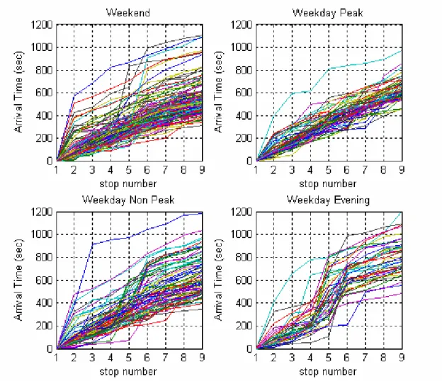
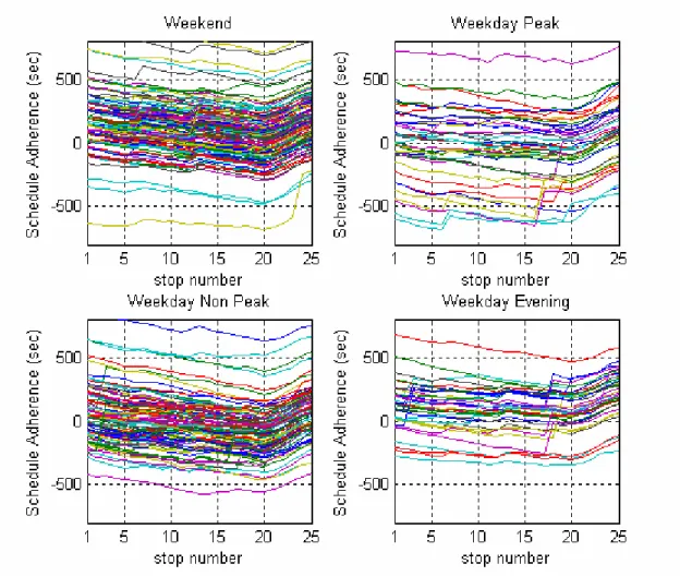
CHAPTER Page 3.2.3.2 Dwell Time...49 3.2.3.3 Schedule adherence ...52 3.3 DATA CHARACTERISTICS...52 3.3.1 Arrival Time... 53 3.3.2 Dwell Time... 61 3.3.3 Schedule Adherence... 73 3.4 CONCLUDING REMARKS...82 IV MODEL DEVELOPMENT ...84
4.1 HISTORICAL DATA BASED MODELS ...89
4.2 MULTI LINEAR REGRESSION MODELS ...91
4.3 ARTIFICIAL NEURAL NETWORK (ANN) MODELS ...104
4.3.1 Structure of Artificial Neural Network (ANN) Models ... 104
4.3.2 Selecting Input Variables ... 106
4.3.3 Selecting the Training Functions ... 109
4.3.4 Selecting the Learning Functions... 114
4.3.5 Number of Neurons... 119
4.4 CONCLUDING REMARKS...121
V MODEL EVALUATION...123
5.1 MAPE OF THE HISTORICAL DATA BASED MODELS ...123
5.2 THE MAPE OF REGRESSION MODELS ...129
5.3 MAPE OF ARTIFICIAL NEURAL NETWORK MODELS ...133
5.4 EVALUATION OF PREDICTION MODELS ...139
5.5 MODEL COMPARISON ...142
5.6 CONCLUDING REMARKS...146
VI PREDICTION INTERVAL, THE PROBABILITY OF A BUS BEING ON TIME, AND REAL-TIME APPLICATION ...148
6.1 PREDICTION INTERVAL...149
6.1.1 Bootstrap Technique ... 149
6.1.2 Result of the Prediction Interval of Bus Arrival Time ... 151
6.2 PROBABILITY OF A BUS BEING ON TIME ...156
6.2.1 Characteristics of Schedule Adherence... 156
6.2.2 Gamma Distribution... 160
6.2.3 Normal Distribution ... 172
6.3 REAL-TIME APPLICATION...182
CHAPTER Page
6.3.2 Real-Time Service... 185
6.3.2.1 Real-Time Prediction vs. Real-Time Service...185
6.3.2.2 Simulation of Real-time Prediction Model and Real-time Service Model...187
6.4 CONCLUDING REMARKS...189
VII CONCLUSIONS ...191
7.1 SUMMARY...191
7.2 Bus Arrival Time Prediction Models...191
7.2.1 Prediction Intervals of Bus Arrival Time... 192
7.2.2 Probability of a Bus Being On-Time ... 192
7.3 CONCLUSIONS ...192
7.3.1 Bus Arrival Time Prediction Models ... 192
7.3.2 Prediction Interval of Bus Arrival Time ... 193
7.3.3 Probability of a Bus Being On-Time ... 193
7.4 FUTURE STUDY...193 GLOSSARY...195 NOTATION ...198 REFERENCES...200 APPENDIX A ...209 APPENDIX B ...214 APPENDIX C ...254 VITA ...278
LIST OF FIGURES
Page
FIGURE 1-1 Framework for Research ...8
FIGURE 2-1 Schematic Display of an AVL System Used in Transit Agencies ...13
FIGURE 2-2 Current Use of AVL Location Technologies ...17
FIGURE 2-3 Twenty Four Satellites of GPS...19
FIGURE 2-4 Calculation of Position, Speed, and Time Using Four Satellites ...19
FIGURE 3-1 Map of Route 60 Running in Houston. ...29
FIGURE 3-2 Map of Route 60 Running in the Test Bed 1 (Downtown) ...30
FIGURE 3-3 Map of Route 60 Running in the Test Bed 2 (North Area)...31
FIGURE 3-4 GPS Measurement Errors...39
FIGURE 3-5 Backward Data Error...40
FIGURE 3-6 Modification of Missing Data ...43
FIGURE 3-7 Modification of Off Route/Road Data ...45
FIGURE 3-8 Illustration of Modifying Off Route/Road Error...46
FIGURE 3-9 Modification of Backward Data...47
FIGURE 3-10 Calculating Arrival Time at Bus Stop ...49
FIGURE 3-11 Calculating Dwell Time at Bus Stop...51
FIGURE 3-12 Arrival Time by Time Period of the Test Bed 1 (Downtown) ...54
FIGURE 3-13 Arrival Time by Time Period of the Test Bed 2 (North Area)...57
Page
FIGURE 3-15 Dwell Time by Time Period of the Test Bed 2 (North Area) ...66
FIGURE 3-16 Schedule Adherence by Time Period of the Test Bed 1 (Downtown) ...74
FIGURE 3-17 Schedule Adherence by Time Period of the Test Bed 2 (North Area)...77
FIGURE 4-1 Arrival Time, Link Travel Time and Dwell Time ...90
FIGURE 4-2 Input-Output Structure of the ANN Models ...105
FIGURE 4-3 Average MAPE by Different Number of Neurons...121
FIGURE 5-1 MAPE Result of Historical Data Based Models of the Test Bed 1 by Time Period (Downtown)...126
FIGURE 5-2 MAPE Result of Historical Data Based Models of the Test Bed 2 by Time Period (North Area) ...127
FIGURE 5-3 MAPE Result of Historical Data Based Models of the Test Bed 1 by Model (Downtown) ...128
FIGURE 5-4 MAPE Result of Historical Data Based Models of the Test Bed 2 by Model (North Area)...128
FIGURE 5-5 MAPE Result of Regression Models of the Test Bed 1 by Time Period (Downtown) ...131
FIGURE 5-6 MAPE Result of Regression Models of the Test Bed 2 by Time Period (North Area)...131
FIGURE 5-7 MAPE Result of Regression Models of the Test Bed 1 by Model (Downtown) ...132
FIGURE 5-8 MAPE Result of Regression Models of the Test Bed 2 by Model (North Area) ...133
FIGURE 5-9 MAPE Result of Artificial Neural Network Models of the Test Bed 1 by Time Period (Downtown) ...136
Page FIGURE 5-10 MAPE Result of Artificial Neural Network Models of the Test
Bed 2 by Time Period (North Area)...137
FIGURE 5-11 MAPE Result of Artificial Neural Network Models of the Test Bed 1 by Model (Downtown)...138
FIGURE 5-12 MAPE Result of Artificial Neural Network Models of the Test Bed 2 by Model (North Area) ...138
FIGURE 5-13 MAPE of Prediction Models of the Test Bed 1 (Downtown) ...140
FIGURE 5-14 Average MAPE of Prediction Models of the Test Bed 2 (North Area)...140
FIGURE 5-15 Average MAPE of Prediction Models of the Test Bed 1 (Downtown) ...141
FIGURE 5-16 Average MAPE of Prediction Models of the Test Bed 2 (North Area)...141
FIGURE 6-1 A Schematic Diagram of a Bootstrap Technique...150
FIGURE 6-2 Prediction Interval of Bus Arrival Time ...154
FIGURE 6-3 Prediction Interval by ANN Models and Regression Models...156
FIGURE 6-4 Schedule Adherence of Non-Clustering...158
FIGURE 6-5 Schedule Adherence of Weekend ...158
FIGURE 6-6 Schedule Adherence of Weekday Peak...159
FIGURE 6-7 Schedule Adherence of Weekday Non-Peak...159
FIGURE 6-8 Schedule Adherence of Weekday Evening ...160
FIGURE 6-9 Observed and Predicted Schedule Adherence by Gamma Distribution (Non-Clustering) ...170
FIGURE 6-10 Observed and Predicted Schedule Adherence by Gamma Distribution (Weekend)...170
Page FIGURE 6-11 Observed and Predicted Schedule Adherence by Gamma
Distribution (Weekday Peak) ...171
FIGURE 6-12 Observed and Predicted Schedule Adherence by Gamma Distribution (Weekday Non-Peak)...171
FIGURE 6-13 Observed and Predicted Schedule Adherence by Gamma Distribution (Weekday Evening) ...172
FIGURE 6-14 Observed and Predicted Schedule Adherence by Normal Distribution (Non-Clustering) ...180
FIGURE 6-15 Observed and Predicted Sschedule Adherence by Normal Distribution (Weekend)...180
FIGURE 6-16 Observed and Predicted Schedule Adherence by Normal Distribution (Weekday Peak) ...181
FIGURE 6-17 Observed and Predicted Schedule Adherence by Normal Distribution (Weekday Non-Peak)...181
FIGURE 6-18 Observed and Predicted Schedule Adherence by Normal Distribution (Weekday Evening) ...182
FIGURE 6-19 Process of Real-Time Prediction...184
FIGURE 6-20 Real-time Prediction Model vs. Real-time Service Model...186
FIGURE 6-21 Real-Time Service Availability...188
FIGURE C- 1 Schedule Adherence of Non-Clustering (stop 1) ...255
FIGURE C- 2 Schedule Adherence of Non-Clustering (stop 2) ...255
FIGURE C- 3 Schedule Adherence of Non-Clustering (stop 3) ...256
FIGURE C- 4 Schedule Adherence of Non-Clustering (stop 4) ...256
FIGURE C- 5 Schedule Adherence of Non-Clustering (stop 5) ...257
Page
FIGURE C- 7 Schedule Adherence of Non-Clustering (stop 7) ...258
FIGURE C- 8 Schedule Adherence of Non-Clustering (stop 8) ...258
FIGURE C- 9 Schedule Adherence of Non-Clustering (stop 9) ...259
FIGURE C- 10 Schedule Adherence of Weekend (stop 1) ...259
FIGURE C- 11 Schedule Adherence of Weekend (stop 2) ...260
FIGURE C- 12 Schedule Adherence of Weekend (stop 3) ...260
FIGURE C- 13 Schedule Adherence of Weekend (stop 4) ...261
FIGURE C- 14 Schedule Adherence of Weekend (stop 5) ...261
FIGURE C- 15 Schedule Adherence of Weekend (stop 6) ...262
FIGURE C- 16 Schedule Adherence of Weekend (stop 7) ...263
FIGURE C- 17 Schedule Adherence of Weekend (stop 8) ...263
FIGURE C- 18 Schedule Adherence of Weekend (stop 9) ...263
FIGURE C- 19 Schedule Adherence of Weekday Peak (stop 1) ...264
FIGURE C- 20 Schedule Adherence of Weekday Peak (stop 2) ...264
FIGURE C- 21 Schedule Adherence of Weekday Peak (stop 3) ...265
FIGURE C- 22 Schedule Adherence of Weekday Peak (stop 4) ...265
FIGURE C- 23 Schedule Adherence of Weekday Peak (stop 5) ...266
FIGURE C- 24 Schedule Adherence of Weekday Peak (stop 6) ...266
FIGURE C- 25 Schedule Adherence of Weekday Peak (stop 7) ...267
FIGURE C- 26 Schedule Adherence of Weekday Peak (stop 8) ...267
Page
FIGURE C- 28 Schedule Adherence of Weekday Non-Peak (stop 1) ...268
FIGURE C- 29 Schedule Adherence of Weekday Non-Peak (stop 2) ...269
FIGURE C- 30 Schedule Adherence of Weekday Non-Peak (stop 3) ...269
FIGURE C- 31 Schedule Adherence of Weekday Non-Peak (stop 4) ...270
FIGURE C- 32 Schedule Adherence of Weekday Non-Peak (stop 5) ...270
FIGURE C- 33 Schedule Adherence of Weekday Non-Peak (stop 6) ...271
FIGURE C- 34 Schedule Adherence of Weekday Non-Peak (stop 7) ...271
FIGURE C- 35 Schedule Adherence of Weekday Non-Peak (stop 8) ...272
FIGURE C- 36 Schedule Adherence of Weekday Non-Peak (stop 9) ...272
FIGURE C- 37 Schedule Adherence of Weekday Evening (stop 1)...273
FIGURE C- 38 Schedule Adherence of Weekday Evening (stop 2)...273
FIGURE C- 39 Schedule Adherence of Weekday Evening (stop 3)...274
FIGURE C- 40 Schedule Adherence of Weekday Evening (stop 4)...274
FIGURE C- 41 Schedule Adherence of Weekday Evening (stop 5)...275
FIGURE C- 42 Schedule Adherence of Weekday Evening (stop 6)...275
FIGURE C- 43 Schedule Adherence of Weekday Evening (stop 7)...276
FIGURE C- 44 Schedule Adherence of Weekday Evening (stop 8)...276
LIST OF TABLES
Page
TABLE 2-1 The Advantages and Disadvantages by Location Technologies...16
TABLE 3-1 Distance between Stops in the Test Bed 1 (Downtown)...32
TABLE 3-2 Distance between Stops in the Test Bed 2 (North Area)...33
TABLE 3-3 Number of Training Data Sets and Test Data Sets for the Test Bed 1 (Downtown) ...35
TABLE 3-4 Number of Training Data Sets and Test Data Sets for the Test Bed 2 (North Area)...35
TABLE 3-5 Structure of AVL Data ...37
TABLE 3-6 Numbers of Modified Data ...42
TABLE 3-7 Number of Observation Data Points by the Missing Duration. ...44
TABLE 3-8 Mean and Standard Deviation of Arrival Time for the Test Bed 1 (Downtown) ...55
TABLE 3-9 Mean and Standard Deviation of Arrival Time for the Test Bed 2 (North Area, Weekend) ...58
TABLE 3-10 Mean and Standard Deviation of Arrival Time for the Test Bed 2 (North Area, Weekday Peak) ...59
TABLE 3-11 Mean and Standard Deviation of Arrival Time for the Test Bed 2 (North Area, Weekday Non-Peak) ...60
TABLE 3-12 Mean and Standard Deviation of Arrival Time for the Test Bed 2 (North Area, Weekday Evening)...61
TABLE 3-13 Mean and Standard Deviation of Dwell Time for the Test Bed 1 (Downtown) ...64
TABLE 3-14 Total and Average Dwell Time by the Time Period for the Test Bed 1 (Downtown) ...65
Page TABLE 3-15 Number of Long Dwell Time by the Time Period for the Test
Bed 1 (Downtown) ...66
TABLE 3-16 Mean and Standard Deviation of Dwell Time for the Test Bed 2 (North Area, Weekend) ...68
TABLE 3-17 Mean and Standard Deviation of Dwell Time for the Test Bed 2 (North Area, Weekday Peak) ...69
TABLE 3-18 Mean and Standard Deviation of Dwell Time for the Test Bed 2 (North Area, Weekday Non-Peak) ...70
TABLE 3-19 Mean and Standard Deviation of Dwell Time for the Test Bed 2 (North Area, Weekday Evening)...71
TABLE 3-20 Total and Average Dwell Time by the Time Period for the Test Bed 2 (North Area)...72
TABLE 3-21 Number of Long Dwell Time by the Time Period for the Test Bed 2 (North Area)...73
TABLE 3-22 Mean and Standard Deviation of Schedule Adherence for the Test Bed 1 (Downtown) ...76
TABLE 3-23 Mean and Standard Deviation of Schedule Adherence for the Test Bed 2 (North Area, Weekend)...79
TABLE 3-24 Mean and Standard Deviation of Schedule Adherence for the Test Bed 2 (North Area, Weekday Peak)...80
TABLE 3-25 Mean and Standard Deviation of Schedule Adherence for the Test Bed 2 (North Area, Weekday Non-Peak)...81
TABLE 3-26 Mean and Standard Deviation of Schedule Adherence for the Test Bed 2 (North Area, Weekday Evening) ...82
TABLE 4-1 Model Specifications...85
TABLE 4-2 Model Structure of the Test Bed 1 (Downtown)...87
Page
TABLE 4-4 Correlation Coefficients of the Test Bed 1 (Downtown) ...91
TABLE 4-5 Correlation Coefficients of the Test Bed 2 (North Area)...92
TABLE 4-6 Stepwise Regression of the Test Bed 1 (Downtown)...93
TABLE 4-7 Stepwise Regression of the Test Bed 2 (North Area) ...94
TABLE 4-8 MAPE for Different Linear Regression Models of the Test Bed 1 (Downtown) ...97
TABLE 4-9 MAPE for Different Linear Regression Models of the Test Bed 2 (North Area, Non-Clustering) ...98
TABLE 4-10 MAPE for Different Linear Regression Models of the Test Bed 2 (North Area, Weekend) ...99
TABLE 4-11 MAPE for Different Linear Regression Models of the Test Bed 2 (North Area, Weekday Peak) ...100
TABLE 4-12 MAPE for Different Linear Regression Models of the Test Bed 2 (North Area, Weekday Non-Peak) ...101
TABLE 4-13 MAPE for Different Linear Regression Models of the Test Bed 2 (North Area, Weekday Evening)...102
TABLE 4-14 Best Regression of the Test Bed 1 (Downtown) ...103
TABLE 4-15 Best Regression of the Test Bed 2 (North Area)...104
TABLE 4-16 MAPE of Artificial Neural Network Models of the Test Bed 1 (Downtown, Non-Clustering)...107
TABLE 4-17 MAPE of Artificial Neural Network Models of the Test Bed 2 (North Area, Non-Clustering) ...108
TABLE 4-18 Running Time of Artificial Neural Network Models...108
TABLE 4-19 Lists of Training Functions ...110
TABLE 4-20 Running Time by Training Function of the Test Bed 1 (Downtown) ...110
Page TABLE 4-21 Average MAPE of Different Training Functions of the Test Bed
1 (Downtown) ...111 TABLE 4-22 Running Time by Training Function of the Test Bed 2 (North
Area)...112 TABLE 4-23 Average MAPE of Different Training Functions...113 TABLE 4-24 Lists of Training Functions ...115 TABLE 4-25 Running Time by Learning Functions of the Test Bed 1
(Downtown) ...116 TABLE 4-26 Average MAPE of Different Learning Functions for the Test
Bed 1 (Downtown) ...117 TABLE 4-27 Running Time by Learning Function of the Test Bed 2 (North
Area)...118 TABLE 4-28 Average MAPE of Different Learning Functions for the Test
Bed 2 (North area)...119 TABLE 4-29 Average MAPE by Different Number of Neurons...120 TABLE 5-1 MAPE for Historical Data Based Models of the Test Bed 1
(Downtown) ...124 TABLE 5-2 MAPE for Historical Data Based Models of the Test Bed 2
(North Area) ...125 TABLE 5-3 MAPE of Multi Linear Regression Models of the Test Bed 1
(Downtown) ...129 TABLE 5-4 MAPE of Multi Linear Regression Models of the Test Bed 2
(North Area) ...130 TABLE 5-5 MAPE of Artificial Neural Network Models of the Test Bed 1
(Downtown) ...134 TABLE 5-6 MAPE of Artificial Neural Network Models of the Test Bed 2
Page
TABLE 5-7 Average MAPE of Prediction Models ...139
TABLE 5-8 Improvement of ANN Models with Respect to Historical Data Based Models and Regression Models...142
TABLE 5-9 ANOVA Table for Non-Clustering Data Set ...145
TABLE 5-10 ANOVA Table for Weekend Data Set...145
TABLE 5-11 ANOVA Table for Weekday Peak Data Set ...145
TABLE 5-12 ANOVA Table for Weekday Non-Peak Data Set...145
TABLE 5-13 ANOVA Table for Weekday Evening Data Set...145
TABLE 5-14 wValues...146
TABLE 5-15 Result of Tukey’s Procedure ...146
TABLE 6-1 Results of Prediction Interval (B=100) ...152
TABLE 6-2 Results of Prediction Interval (B=200) ...153
TABLE 6-3 Results of Prediction Interval (B=1000) ...153
TABLE 6-4 Prediction Interval by ANN Models and Regression Models...155
TABLE 6-5 Mean and Standard Deviation of Schedule Adherence...164
TABLE 6-6 Parameters for Gamma Distribution ...164
TABLE 6-7 Probability and Predicted Frequencies of Non-Clustering...165
TABLE 6-8 Probability and Predicted Frequencies of Weekend ...166
TABLE 6-9 Probability and Predicted Frequencies of Weekday Peak...167
TABLE 6-10 Probability and Predicted Frequencies of Weekday Non-Peak ...168
TABLE 6-11 Probability and Predicted Frequencies of Weekday Evening ...169
Page
TABLE 6-13 Probability and Predicted Frequencies of Weekend ...176
TABLE 6-14 Probability and Predicted Frequencies of Weekday Peak...177
TABLE 6-15 Probability and Predicted Frequencies of Weekday Non-Peak ...178
TABLE 6-16 Probability and Predicted Frequencies of Weekday Evening ...179
TABLE A- 1 Bus Schedule by Bus Stop for the Study Period (Downtown Area, Weekday)...210
TABLE A- 2 Bus Schedule by Bus Stop for the Study Period (Downtown Area, Weekend)...211
TABLE A- 3 Bus Schedule by Bus Stop for the Study Period (North Area, Weekday) ...212
TABLE A- 4 Bus Schedule by Bus Stop for the Study Period (North Area, Weekend) ...213
TABLE B-1 MAPE of ANN Models with Different Training Functions (Batch Training with Weight and Bias Learning Rule) ...215
TABLE B-2 MAPE of ANN Models with Different Training Functions (BFGS Quasi-Newton Backpropagation)...215
TABLE B-3 MAPE of ANN Models with Different Training Functions (Bayesian Regularization) ...216
TABLE B-4 MAPE of ANN Models with Different Training Functions (Powell-Beale Conjugate Gradient Backpropagation)...216
TABLE B-5 MAPE of ANN Models with Different Training Functions (Fletcher-Powell Conjugate Gradient Backpropagation)...217
TABLE B-6 MAPE of ANN Models with Different Training Functions (Gradient Descent Backpropagation) ...217
TABLE B-7 MAPE of ANN Models with Different Training Functions (Gradient Descent with Adaptive Learning Rate Backpropagation) ...218
Page TABLE B-8 MAPE of ANN Models with Different Training Functions
(Levenberg-Marquardt Backpropagation)...218 TABLE B-9 MAPE of ANN Models with Different Training Functions (One
Step Secant Backpropagations)...219 TABLE B-10 MAPE of ANN Models with Different Training Functions
(Resilient Backpropagation)...219 TABLE B-11 MAPE of ANN Models with Different Training Functions
(Sequential Order Incremental Update) ...220 TABLE B- 12 MAPE of ANN Models with Different Training Functions
(Scaled Conjugate Gradient Backpropagation)...220 TABLE B-13 MAPE of ANN Models with Different Training Functions
(Batch Training with Weight and Bias Learning Rule) ...221 TABLE B-14 MAPE of ANN Models with Different Training Functions
(BFGS Quasi-Newton Backpropagation)...222 TABLE B-15 MAPE of ANN Models with Different Training Functions
(Bayesian Regularization) ...223 TABLE B-16 MAPE of ANN Models with Different Training Functions
(Powell-Beale Conjugate Gradient Backpropagation)...224 TABLE B-17 MAPE of ANN Models with Different Training Functions
(Fletcher-Powell Conjugate Gradient Backpropagation)...225 TABLE B-18 MAPE of ANN Models with Different Training Functions
(Gradient Descent Backpropagation) ...226 TABLE B-19 MAPE of ANN Models with Different Training Functions
(Gradient Descent with Adaptive Learning Rate
Backpropagation) ...227 TABLE B-20 MAPE of ANN Models with Different Training Functions
(Levenberg-Marquardt Backpropagation)...228 TABLE B-21 MAPE of ANN Models with Different Training Functions (One
Page TABLE B-22 MAPE of ANN Models with Different Training Functions
(Resilient Backpropagation)...230 TABLE B-23 MAPE of ANN Models with Different Training Functions
(Sequential Order Incremental Update) ...231 TABLE B-24 MAPE of ANN Models with Different Training Functions
(Scaled Conjugate Gradient Backpropagation)...232 TABLE B-25 MAPE of ANN Models with Different Learning Functions
(Conscience Bias Learning Function) ...233 TABLE B-26 MAPE of ANN Models with Different Learning Functions
(Gradient Descent Weight/Bias Learning Function)...233 TABLE B-27 MAPE of ANN Models with Different Learning Functions
(Gradient Descent with Momentum Weight/Bias Learning
Function) ...234 TABLE B-28 MAPE of ANN Models with Different Learning Functions
(Hebb Weight Learning Function) ...234 TABLE B-29 MAPE of ANN Models with Different Learning Functions
(Hebb with Decay Weight Learning Function)...235 TABLE B-30 MAPE of ANN Models with Different Learning Functions
(Instar Weight Learning Function)...235 TABLE B-31 MAPE of ANN Models with Different Learning Functions
(Kohonen Weight Learning Function) ...236 TABLE B-32 MAPE of ANN Models with Different Learning Functions
(LVQ1 Weight Learning Function)...236 TABLE B-33 MAPE of ANN Models with Different Learning Functions
(LVQ2 Weight Learning Function)...237 TABLE B-34 MAPE of ANN Models with Different Learning Functions
(Outstar Weight Learning Function) ...237 TABLE B- 35 MAPE of ANN Models with Different Learning Functions
Page TABLE B- 36 MAPE of ANN Models with Different Learning Functions
(Normalized Perceptron Weight and Bias Learning Function)...238 TABLE B-37 MAPE of ANN Models with Different Learning Functions
(Self-organizing Map Weight Learning Function)...239 TABLE B-38 MAPE of ANN Models with Different Learning Functions
(Widrow-Hoff Weight and Bias Learning Rule)...239 TABLE B-39 MAPE of ANN Models with Different Learning Functions
(Conscience Bias Learning Function) ...240 TABLE B-40 MAPE of ANN Models with Different Learning Functions
(Gradient Descent Weight/Bias Learning Function)...241 TABLE B-41 MAPE of ANN Models with Different Learning Functions
(Gradient Descent with Momentum Weight/bias Learning
Function) ...242 TABLE B-42 MAPE of ANN Models with Different Learning Functions
(Hebb Weight Learning Function) ...243 TABLE B-43 MAPE of ANN Models with Different Learning Functions
(Hebb with Decay Weight Learning Function)...244 TABLE B-44 MAPE of ANN Models with Different Learning Functions
(Instar Weight Learning Function)...245 TABLE B-45 MAPE of ANN Models with Different Learning Functions
(Kohonen Weight Learning Function) ...246 TABLE B-46 MAPE of ANN Models with Different Learning Functions
(LVQ1 Weight Learning Function)...247 TABLE B-47 MAPE of ANN Models with Different Learning Functions
(LVQ2 Weight Learning Function)...248 TABLE B-48 MAPE of ANN Models with Different Learning Functions
(Outstar Weight Learning Function) ...249 TABLE B-49 MAPE of ANN Models with Different Learning Functions
Page TABLE B-50 MAPE of ANN Models with Different Learning Functions
(Normalized Perceptron Weight and Bias Learning Function)...251 TABLE B-51 MAPE of ANN Models with Different Learning Functions
(Self-organizing Map Weight Learning Function)...252 TABLE B-52 MAPE of ANN Models with Different Learning Functions
CHAPTER I
INTRODUCTION
1
One component of Intelligent Transportation Systems (ITS) is Advanced Traveler Information System (ATIS), and a major component of ATIS is providing travel time information by different modes to travelers. The provision of timely and accurate transit arrival time information is important because it attracts additional transit ridership and increases the satisfaction of transit users (1-5).
The cost of electronics and components for ITS has been decreased, and ITS deployment is growing nationwide (6, 7). Automatic Vehicle Location (AVL) Systems, which are a part of ITS, have been adopted by many transit agencies, allowing them to track their transit vehicles in real-time (7). While the provision of real-time information, such as bus location, is relatively straightforward, forecasting transit information, such as when a bus will arrive at a particular location, is significantly more complex. Consequently, the need for predicting transit arrival time using AVL data is increasing. While some
research on this topic has been conducted, there is still important work to be done (8-12).
1.1 STATEMENT OF PROBLEM
1.1.1 Need to Develop a Bus Arrival Time Prediction Model Using AVL Data The increase in the transit ridership and the satisfaction of transit users can be achieved by the provision of current traveler information (1-5). In addition, transit operators can identify vehicles that 1) have fallen behind schedule or 2) are in danger of falling behind schedule, and react in a proactive way. For example, bus priority at traffic signals could
be enabled. Because ITS technologies are deployed nationwide (1, 2, 6, 7), the usage of AVL systems by transit agencies continues to increase (7). Consequently, the need for robust prediction algorithms increases. While there has been some preliminary work in this area, there are a number of questions that need to be considered.
1.1.2 Need to Explicitly Consider Traffic Congestion
In order to predict travel time in an accurate and timely manner, the consideration of traffic conditions is essential, including traffic congestion. The impact of recurrent and non recurrent congestion has been ignored. Lin and Zeng did not consider traffic
congestion because their algorithm was formulated primarily for a rural area and because they did not have a system which measured traffic congestion (9). Ojili used one-minute time zones where a bus can run for one minute (10). After finding the current bus location, he predicted the arrival time by counting the estimated number of one-minute time zones between the current location and the given stop. Because the one-minute time zones could be changed by time period or by traffic condition, the model would have to be recalibrated if traffic conditions change. Because Shalaby and Farhan used a Kalman filtering technique, they assumed that the pattern of link travel time is cyclical (13). In summary, a prediction model that explicitly considers traffic congestion is needed.
1.1.3 Need to Explicitly Consider Dwell Times at Bus Stops
The major difference in predicting bus and auto travel times is that the former needs to consider dwell time at bus stops. However, there has been little research that explicitly considers bus dwell times when predicting transit arrival times. Lin and Zeng used regular global positioning systems (GPS), not differential global positioning systems (DGPS), and their GPS unit provided bus location every forty six seconds. They were not able to measure exact dwell time at stops, and consequently they did not explicitly consider it in their model (9). Similar to the previous argument, Ojili (10) and Wall and Dailey (8) did not consider dwell times when they predicted transit arrival time. Shalaby and Farhan assumed that dwell times increase when a bus arrives late because there
would be more passengers waiting for the bus (13). In addition, they assumed that dwell time is directly proportional to passenger demand and simply multiplied by 2.5 seconds per passenger. However, they did not consider the fact that the bus driver will stay longer to keep to schedule when they arrive early or that the bus driver can stay at bus stops even though there is no passenger. Because dwell time is a function of the behavior of the bus driver and passengers, a model that can explain the uncertainty of the behavior is required. In summary, a prediction model which explicitly considers dwell time at bus stops is needed.
1.1.4 Need to Consider Schedule Adherence
Transit vehicles have a predefined schedule to follow. Because of this requirement, bus drivers may stay longer at bus stops if they are ahead of schedule and/or to pass some stops if they are behind schedule. In other words, bus schedules control the behavior of bus drivers, dwell times at bus stops, and link travel times. Schedule adherence is the difference between schedule time and actual arrival time. A positive value of schedule adherence means that the bus arrives late and negative value means that the bus arrives early. Consequently, a bus arrival time prediction model should consider schedule adherence as an input variable.
1.1.5 Need to Provide Prediction Intervals
Most existing bus arrival time prediction models only provide the mean value of bus arrival time. For example, the information might be that the bus will arrive in 10 minutes. However, prediction errors tend not to be provided. If a prediction interval is provided with the mean value, it should give more useful information for passengers when making their decisions. For example, the information would be that the bus will arrive in 10 minutes plus or minus 1 minute. Rather than providing a point prediction value, an interval prediction value would be more valuable information for transit users.
1.1.6 Need to Provide the Probability of a Bus Being on Time
On-time performance of a bus is very substantial to transit operators because customers use this to measure quality of service. It would be extremely important to identify, in real-time, whether a given bus is on schedule or not. To measure the on-time
performance, the probability of a bus being on time is required. In addition to the prediction interval of bus arrival time, the probability that a given bus is on time is needed to be estimated.
1.2 RESEARCH OBJECTIVES
It is hypothesized that a bus arrival time prediction model considering traffic congestion and dwell time will give a superior result compared to simple conventional prediction models. The objectives of this research are to develop and apply a statistical model to predict bus arrival time using AVL data. Arrival time information can be provided to travelers to help in their decision making and can be used by transit operators to improve their operations. Specific objectives of this research are as follows:
Analyze the characteristics of AVL data, including arrival time, dwell time, and schedule adherence data.
Select reasonable input variables for a bus prediction model.
Cluster input data by time period to implicitly consider traffic congestion. Develop prediction models including historical data based models, multi linear regression models, and artificial neural network models.
Forecast the bus arrival travel time with three developed models. Evaluate these three models in terms of prediction accuracy.
Develop a methodology for identifying the prediction interval of the bus arrival time. Identify a probability function to estimate the probability of a bus being on time.
1.3 RESEARCH FRAMEWORK AND METHODOLOGIES
1.3.1 Perform a Literature Review
Related research reports, journal articles, and Ph. D. dissertations were reviewed. The primary areas of interest are 1) the current state of practice and trends in the provision of traveler information 2) the technology of AVL systems, 3) GPS theory, and 4) the methodology for travel time prediction. The purpose of this task is to ensure that no research relevant to this study is overlooked or inappropriately duplicated.
1.3.2 Collect Data and Define Test Bed
Actual AVL data collected in Houston, Texas, were used as a test bed. The Houston data were collected by Houston Metro buses equipped with DGPS receivers that collect data at 5 seconds intervals. Data were collected over 6 months in 2000 (from June to
November). The test bed is route 60, which runs on a congested corridor in Houston. This DGPS provides time, speed, heading, etc., as well as bus location.
There are two test bed sites: a downtown area corridor and a north area corridor. The first corridor has 9 bus stops and is 1.6 kilometer long. Stop 1 and stop 9 are time check points where bus drivers should keep to scheduled time. The second corridor has 25 bus stops and is 4.26 kilometer long. Stop 6 and stop 20 are time check points. The schedule headway during weekday peak period is about 30 minutes and during the weekday non-peak period and weekends is about 1 hour.
1.3.3 Reduce Data and Correct Errors
There are two types of errors associated with GPS data. The first is noise errors added by the U.S. DOD in order to degrade the accuracy of GPS data. This error was corrected by using DGPS. The second type of error is measurement errors. It is anticipated that some of the bus location data were correspond to off-route locations (i.e. parking lot, refueling station, etc.). In addition, even if the bus is located on the road, there would be errors
associated with its exact location. An additional source of data error would be missing data. Where the data are missing, existing data were used to calculate input data according to distance. Outliers were also identified when the data are located unreasonably far away from the road.
1.3.4 Cluster Data
The transit schedule and congestion for weekday peak hour, non-peak hour, evening, and weekend, are different. It would be expected that dwell time and link travel time would also be different. To account for these differences, data were clustered by time of the week and time of the day.
1.3.5 Develop Prediction Models
A number of modeling techniques were used including a simple statistical model (historical data), a regression model, and an artificial neural network model. In this research, the input variables were be arrival time, dwell time, and schedule adherence at each stop. To consider traffic congestion, schedule adherence was calculated by
subtracting the scheduled data from the actual arrival time. A positive value of schedule adherence means that the bus is delayed at the stop while a negative value means that the bus arrives early. To consider traffic congestion, the link travel times were clustered by time period in task 4. The output variable is arrival time at each stop.
1.3.6 Evaluate Prediction Models
All three model architectures were calibrated. With these calibrated models, the arrival times were predicted. A validation data set was obtained in order to test which model is most appropriate. Predicted arrival times were compared to the observed arrival times from the validation data set. The Mean Absolute Percentage Error (MAPE) was used as the measure of effectiveness (MOE). The MAPE is shown in Equation 1-1. It represents the average percentage difference between the observed value (in this case observed arrival times at a bus stop) and the predicted value (in this case predicted arrival times at
a bus stop). Smaller MAPE means that the model predicts more accurately than other models. % 100 1 − × =
∑
n i o o i y y y n MAPE (1-1) where,yi = Predicted value (i.e. arrival time at given transit stop);
yo= Observed value (i.e. arrival time at given transit stop);
n = The number of data considered.
1.3.7 Identify the Prediction Interval of the Bus Arrival Time
The model with the smallest MAPE is chosen for the prediction model for the bus arrival time. With the selected model, prediction intervals on these estimates were provided. If ANN models are chosen for the outperformed model, the conventional method for finding prediction interval is not appropriate. In that case, the bootstrap method, which is a statistical method that provides prediction intervals for non-parametric models, was used. In order to statistically test the differences in mean and variance of the three different models, one of several pairwise comparison methods, such as Tukey’s procedure was used.
1.3.8 Identify the Probability of a Bus Being on Time
The probability density function of schedule adherence was identified. To determine which distribution was the best fit for schedule adherence, a chi-squared goodness-of-fit test was used. After identifying the best fit probability density function, the probability of a bus being on time, being ahead schedule, and being behind schedule were able to be estimated.
FIGURE 1-1 Framework for Research
1.4 CONTRIBUTION OF THE RESEARCH
Providing travel time information is a major component of ATIS. With the deployment of ATIS, the provision of traveler information can extend the ridership and increase the
satisfaction of transit users. Many transit agencies have adopted Automatic Vehicle Location (AVL) Systems and track their transit vehicles in real-time. The need for a model or technique to predict transit arrival time using AVL data is increasing. While some research on this topic has been conducted, there is still important work to be done.
To provide accurate and timely traveler information, consideration of the traffic conditions is essential. However, recent research has not fully considered traffic congestion and dwell times at bus stops, which are critical factors for predicting bus arrival time. This research can provide more accurate prediction of bus arrival time considering traffic congestion and dwell time. In addition to the mean value of arrival time, prediction interval information was provided. This would be more reliable information for both passengers and transit agencies, leading to better operation.
1.5 ORGANIZATION OF THE RESEARCH
This dissertation is organized into eight chapters. Chapter I is an introduction to the research and discusses the background of the problem, statement of the problem, research objectives, research methodology, contribution of the research, and the organization of the dissertation. Chapter II presents a literature reviews on advanced traveler information systems, automatic vehicle location systems, global positioning systems, travel time prediction models, and bus arrival time prediction models. Chapter III describes the details of the test bed and the reduction of the data. Chapter IV
describes and graphically depicts the characteristics of the input variables. The development of three bus arrival time prediction models is included in chapter IV, including a historical data based model, a multi linear regression model, and an artificial neural network model. Chapter V discusses the evaluation of the three prediction models. In addition to this, the statistical test for model comparison is conducted in this chapter. Chapter VI discusses the prediction interval of bus arrival time and the probability that a bus is behind schedule. Chapter VII provides contributions and recommendations based on the research. Suggestions for further research are also included in this chapter. The
references are followed by a glossary of frequently used terms and acronyms. The appendices also include the results of artificial neural network models with different training and learning functions.
CHAPTER II
LITERATURE REVIEW
2
2.1 ADVANCED TRAVELER INFORMATION SYSTEMS (ATIS)
2.1.1 Types of Traveler Information Systems
A traveler who wants to move from point A to point B faces a number of decisions including: what transportation mode do I need to use, what time do I need to depart, what transit route or what road do I need to use, etc. Traveler information systems help travelers to make decisions regarding mode, route, and departure time. There are three types of traveler information, and they can be categorized according to the time at which information is provided: pre-trip information, terminal/wayside information, and in-vehicle information (1).
Pre-trip information, which is provided before the trip begins, includes transit routes, maps, schedules, fares, park-and-ride lot locations, points of interest, and weather. The information can be distributed by touch-tone telephone, Internet, kiosks, personal pagers, hand-held data receivers, and cable television.
In-terminal/Wayside transit information is provided to transit riders who are already en-route. The information can be distributed by electronic signs, interactive information kiosks, and closed-circuit television monitors.
In-vehicle transit information is provided to transit users while they are in the transit vehicle. Many transit agencies use automated annunciators and in-vehicle displays to provide information about audible and visual next stop, intersection, and transfer point.
2.1.2 Importance of the Provision of Traveler Information
There are a number of reasons why travelers do not use transit. It has been shown that the lack of information and the lack of schedule reliability discourage transit use (1-3, 14). It is hypothesized that if reliable transit information could be provided, travelers would be more likely to use transit. Additionally, it has also been shown that out-of-vehicle waiting time is more critical than in-out-of-vehicle travel time when users perceive the quality of transit service (4). Therefore, a reduction in the uncertainty of out-of-vehicle waiting time would enhance the satisfaction of transit users. If accurate arrival time forecasts could be provided to transit users through ATIS, then this uncertainty would be reduced and ridership would increase. Consequently, the provision of accurate and timely traveler information encourages positive attitudes toward transit resulting in increased ridership (1-3, 5). The provision of traveler information is important for transit operators because it not only attracts additional ridership but also increases the
satisfaction of current users (1-5). In addition, transit operators can identify vehicles that 1) have fallen behind schedule or 2) are in danger of falling behind schedule, and react in a proactive way. For example, bus priority at traffic signals could be enabled.
2.1.3 Real-time Information
A recent trend, which is directly related to the advances in ITS technologies, is the provision of real-time transit information (2, 15). Real-time transit information includes: transit vehicle arrival time, transit vehicle departure time, current transit vehicle location, speed, and delay. Real-time information is very valuable to transit users because 1) the knowledge of the arrival time can reduce their anxiety related to waiting, and 2) the transit riders can decide whether to wait at transit stops or seek another mode of travel (5). To provide better service for transit patrons, many transit agencies are planning or providing real-time information (6, 16). Real-time data are obtained from Automatic Vehicle Location (AVL) Systems or Automatic Vehicle Identification (AVI) devices, and it can be provided as real-time traveler information directly. However, more commonly the data are processed in order to provide information such as bus arrival
time, link travel time, delay, etc., because this is the type of information most valuable to transit users.
2.2 AUTOMATIC VEHICLE LOCATION (AVL) SYSTEMS
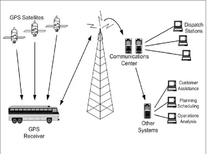
Automatic Vehicle Location (AVL) Systems are computer-based vehicle tracking systems. They are also referred to as Automatic Vehicle Monitoring (AVM) Systems or Automatic Vehicle Location and Control (AVLC) Systems (1). They are used in transit, trucking fleets, police cars, ambulances, and for military purposes, and their use in transit continues to grow (1). FIGURE 2-1 shows the schematic display of an AVL system used in transit agencies (2).
2.2.1 Benefits of AVL Systems
The benefits of AVL systems are as follows:
1) they collect real-time information which can be provided to the public, 2) they improve schedule reliability,
3) they reduce operating and maintenance costs, 4) they improve service efficiency,
5) they enhance safety and security, and
6) the transit agencies can respond more quickly to emergency situations (17-19). The benefits of AVL systems have been well documented. Schedule adherence
improved by 23% in Baltimore, 12.5% in Kansas City, 8.5% in Hamilton, Ontario, and 4.4% in Milwaukee after AVL installation (18, 20). Operating costs were reduced $500,000/year in Kansas City, and $45,000/year in London, Ontario (21). Paratransit ridership increased by 17.5% and paratransit passenger waiting time decreased by 50% in Winston-Salem, North Carolina (21).
2.2.2 Uses of AVL Systems
The first use of AVL technology in transit was in London, England in the late 1950s, and the first use in the United States was in Chicago in the late 1960s (6). A number of transit systems in North America and abroad began to plan for and implement AVL systems during the 1980s (6).
According to the research of Casey in 2002, 322 transit agencies are either operating, implementing, or planning/ testing/ demonstrating AVL systems (16). The number of transit agencies used AVL systems increased by four hundred percent as compared to earlier studies in 1995 (7, 16, 22). An increasing number of transit agencies are planning to install AVL systems because the cost of AVL systems has rapidly dropped (6, 18-22).
2.2.3 Technologies of AVL Systems
AVL systems consist of two technologies, location technology and data transmission technology. “Location technology is used to measure actual real-time position of each vehicle, and data transmission technology is used to relay the information to a central location” (1).
2.2.3.1LocationTechnology
Location technology includes dead-reckoning, signpost and odometer, global positioning systems (GPS), differential GPS (DGPS), etc. For transit vehicle, a single location technology is usually insufficient for determining position. For instance, tall buildings block the signals and result in multi-path errors. Therefore, the primary location
technology is supplemented with another location technology (1). TABLE 2-1 details the advantages and disadvantages of different location technologies.
Dead-reckoning is the most self-determined form of location technology. The transit vehicle determines its own location without the help of external technologies. First, the transit vehicle is told its starting point. The vehicle measures the traveled distance from the starting point by reading the odometer. Then the vehicle determines the traveled direction by compass headings. Dead-reckoning location technology is seldom used by itself because the equipment has to be reset frequently from a known location. Dead-reckoning is usually supplemented by one of other location technologies like signpost or GPS (1). It is relatively inexpensive, but the accuracy degrades with distance traveled (23).
Signpost and odometer uses a series of radio beacons placed along the bus routes. The beacons send a low power signal and the signal is detected by a receiver on the transit vehicle. Then the transit vehicle reports its position to dispatch according to the traveled distance, which is taken from the odometer (1). This technology requires low in-vehicle
cost and it is well established and proven. However, additional installation is required with route changes and it can not track the vehicle when a bus is off-route (1, 23). Global positioning systems (GPS) determine the position using the signals which are transmitted from up to 24 satellites. GPS works anywhere the satellites reach, and it is much more robust than other location technologies. However, satellite signals do not reach underground and they can be interrupted by tall buildings or foliage. Where these problems happen, signpost and odometer can supplement the GPS (1).
The U.S. Department of Defense (DOD) intentionally degraded the accuracy of GPS for safety reason. To correct this interruption, an additional (differential) correction was added and this system is called Differential GPS (DGPS) (1).
TABLE 2-1 The Advantages and Disadvantages by Location Technologies
Type Advantages Disadvantages
Dead reckoning
Relatively inexpensive Self-contained on vehicle (no infrastructure costs)
Only odometer needed (if on-route is assumed)
Accuracy degrades with distance traveled (errors can accumulate between known locations)
- Requires direction indicator and maybe map matching for off-route use
Corrupted by uneven road surfaces, steep hills, or magnetic interference
Signpost and odometer
Low in-vehicle cost
No blind spots or interference Repeatable accuracy
Requires well-equipped infrastructure No data outside of deployed infrastructure Frequency of updates depends on density of signpost
GPS
Moderately accurate Global coverage
Moderate cost per vehicle
Signal attenuation by foliage and tunnels Subject to multi-path errors
DGPS
Very accurate
Moderate cost per vehicle
Signal attenuation by foliage and tunnels Subject to multi-path errors
Must be within range of differential signal Differential correction must be updated frequently
In the early 1990s, more than 60 percent of transit agencies choose signpost and
odometer systems as their AVL location technology (7). However, by 1999, it was found that more than 80 percent of transit agencies choose GPS/DGPS technology (7).
FIGURE 2-2 shows the current use of AVL location technologies. The accuracy of AVL systems is critical for transit applications and, ultimately, to increase ridership (6). The use of GPS eliminates the concern about accuracy of information from ground-based AVL systems using odometer readings (6).
GPS/DGPS 86% Other 2% Loran-C 1% Dead reckoning 1% Signpost and odometer 10% GPS/DGPS Signpost and odometer Loran-C Dead reckoning Other
FIGURE 2-2 Current Use of AVL Location Technologies
2.2.3.2Data Transmission Technology
Position information, regardless of which location technology is adopted, is usually stored on the transit vehicle for some period of time. The information is relayed to the
dispatch center in raw form or is processed on-board the vehicle. The two most common data transmission technology are polling and exception reporting (1, 18).
With polling technology, the computer at the dispatch center asks each bus for its location at regular intervals. The accuracy of location is a function of how often the transit vehicle is polled. In addition, the number of radio frequencies which are available in urban areas is limited. Due to this reason, many transit agencies have chosen another technology, exception reporting (1).
Under the exception reporting method, each bus reports its location at a few specified locations or when the bus is found to be off-schedule by some pre-defined tolerance. Exception reporting requires each transit vehicle to know not only its position but also its scheduled position. Many agencies combine the polling and exception reporting methods (1, 18).
2.3 GLOBAL POSITIONING SYSTEMS (GPS)
GPS is a satellite-based navigation system which is funded and controlled by the U.S. Department of Defense (DOD) (23). Even though it was intended for military use, the system has been available for civilian applications world-wide since the 1980s (24). The GPS consists of 24 satellites (see FIGURE 2-3) and transmits the estimated position, velocity, and current time to GPS receivers. To compute position, velocity, and current time, signals from at least four satellites are used (see FIGURE 2-4).
FIGURE 2-3 Twenty Four Satellites of GPS
2.3.1 Accuracy of GPS
GPS has two positioning services, Precise Positioning Service (PPS) and Standard Positioning Service (SPS). PPS is used by authorized users such as U.S. and Allied military while SPS is used by civilian users worldwide (24). For security reasons the DOD intentionally degraded SPS accuracy. The accuracy of PPS was within 22 meters, and the accuracy of SPS was within 100 meters (24). To improve the accuracy of SPS, an additional correction (differential) signal was added, and is called Differential GPS (DGPS) (25). The accuracy of DGPS was better than 10 meters (23).
The SPS accuracy was dramatically improved when the US military removed the
intentional degradation to the signal on May 1, 2000 (25). Currently the accuracy of PPS and SPS are the same. The current accuracy of GPS is between 10 and 20 meters, and that of DGPS is between 3 and 5 meters (18, 26).
2.3.2 Use of GPS in Transportation
While traditional methods of data collection techniques in transportation are burdensome, time consuming, and error prone, GPS provides better accuracy, consistency, automation, and easier integration between collected data and the data based on GIS (27-28).
Because of the advantages of GPS, a number of studies on data collection using GPS have been conducted (28-32). They used GPS to collect travel time, speed, route choice, and travel surveys. They have shown that the use of GPS for collecting data is easier and more accurate than traditional methods (28-32).
2.4 TRAVEL TIME PREDICTION MODELS
The accurate prediction of link travel time is critical to ITS transit applications. With the development of Advanced Travelers Information Systems (ATIS), the importance of the short-term travel time prediction has increased markedly (33). A number of prediction models, including historical data based models, regression models, time series models
and neural network models, have been developed over the years by various transit agencies.
2.4.1 Historical Data Based Models
Historical data based models predict travel time for a given time period using the average travel time for the same time period obtained from a historical data base. These models assume that traffic patterns are cyclical and the ratio of the historical travel time on a specific link to the current travel time reported in real-time will remain constant (34). The procedure requires an extensive set of historical data and it is difficult to install the system in a new setting (34). Real-time models assume that the most recently
observed transit travel times will stay consistently into the future. Chen et al developed a prediction algorithm that combined these two approaches. First a historical data base was used to obtain estimated travel time. This time was subsequently adjusted as real-time location data are obtained (35).
2.4.2 Regression Models
Regression models are conventional approaches for predicting travel time (36).
Regression models predict a dependent variable with a mathematical function formed by a set of independent variables (12). To establish a regression model, the dependent variables need to be independent. This requirement limits the applicability of the regression model to the transportation areas because variables in transportation systems are highly inter-correlated (12).
2.4.3 Time Series Models
Time series models assume that the historical traffic patterns will remain the same in the future. The accuracy of Time series models is a function of the similarity between the real-time and historical traffic patterns (12). Variation in historical data or changes in the relationship between historical data and real-time data could significantly cause inaccuracy in the prediction results (37). D’Angelo used a non-linear time series model
to predict a corridor travel time on a highway (37). He compared two cases: the first model used only speed data as a variable, while the second model used speed, occupancy, and volume data to predict travel time. It was found that the single variable model using speed was better than the multivariable prediction model.
2.4.4 Kalman Filtering Models
Kalman filtering models have been used extensively in travel time prediction research (12, 38). Chen and Chien (33, 39-40) and Wall and Dailey (8, 41) used Kalman filtering techniques to predict auto travel time. The Kalman filtering model has the potential to adapt to traffic fluctuation with time-dependent parameters (12). These models are effective in predicting travel time one or two time periods ahead, but they deteriorate with multiple time steps (42). Park and Rilett compared neural network models with other prediction models including Kalman filtering techniques to predict freeway link travel time. While the average mean absolute percentage error (MAPE) of neural network models changed from 8.7 for one time period to 16.1 for 5 time periods, that of Kalman filtering changed from 5.7 to 20.1 (42)
2.4.5 Artificial Neural Network Models
Due to their ability to solve complex non-linear relationships, artificial neural network models (ANNs) have been developed for transportation since the early 1990s (43-50). ANN models had better results than those of existing link travel time techniques,
including a Kalman filtering model, an exponential smoothing model, a historical profile, and a real-time profile (42, 51-52). In addition, ANN model showed better performance than historical average and autoregressive integrated moving average (ARIMA) models to predict short-term traffic flow (34). While other models are dependent on cyclical traffic data patterns or need independence between dependent and independent variables, ANNs do not require that variables be uncorrelated and/or that they have a cyclic pattern (41).
ANNs emulate the learning process of the human brain (53). They are good at pattern recognition, prediction, classification, etc. ANNs have two stages, training and testing. During the training stage, inductive learning principles are used to learn patterns from a training set data. There are two types of learning processes used: unsupervised and supervised learning. In unsupervised learning, the network attempts to classify the training set data into different groups based on input patterns. In supervised learning, the desired output from output layer neurons is known, and the network adjusts the weight of connections between neurons to produce the desired output (54). During this process, the error in the output is propagated back from one layer to the previous layer by
adjusting the weights of the connections (54). This is called the back-propagation method, which is the most frequently used technique in transportation applications (34, 45, 49, and 54). The learning process of ANNs can be continuous so that the models can adapt to changes in environmental characteristics. In other words, ANN models can be considered dynamic prediction models because they can be updated and modified using new online data (41).
2.5 BUS TRAVEL TIME PREDICTION MODELS
In the previous section, travel time prediction models which have been developed were discussed. The travel time prediction models focused on travel time for passenger cars. In this section, travel time prediction models for transit vehicles are reviewed.
In the context of input data source, various types of data source including loop detectors, microwave detectors, radar, etc., have been used. Travel time data can be obtained from these data sources. However, it is not realistic that the entire urban roadway network would be covered by such devices. Thanks to the development of technologies, more reliable data from specific devices that can track the vehicles such as GPS can be collected (33). Recently, a few cities have conducted research on predicting transit travel time using AVL data.