International Journal of Prognostics and Health Management, ISSN 2153-2648, 2019 009 1
A New Hybrid Prognostic Methodology
Omer F. Eker1, Fatih Camci2*, and Ian K. Jennions3 1Artesis, Gebze, Kocaeli, Turkey
[email protected] 2Amazon, Austin TX USA
3Integrated Vehicle Health Management Centre, Bedfordshire, UK [email protected]
ABSTRACT
Methodologies for prognostics usually centre on physics-based or data-driven approaches. Both have advantages and disadvantages, but accurate prediction relies on extensive data being available. For industrial applications this is very rarely the case, and hence the chosen method’s performance can deteriorate quite markedly from optimal. For this reason, a hybrid methodology, merging physics-based and data-driven approaches, has been developed and is reported here. Most, if not all, hybrid methods apply physics-based and data-driven approaches in different steps of the prognostics process (i.e. state estimation and state forecasting). The presented technique combines both methods in forecasting, and integrates the short-term prediction of a physics-based model with the longer-term projection of a similarity-based data-driven model, to obtain remaining useful life estimation. The proposed hybrid prognostic methodology has been tested on two engineering datasets, one for crack growth and the other for filter clogging. The performance of the presented methodology has been evaluated by comparing remaining useful life estimations obtained from both hybrid and individual prognostic models. The results show that the presented methodology improves accuracy, robustness and applicability, especially in the case of minimal data being available.
1.INTRODUCTION
Prognostics and Health Management (PHM) is a comprehensive technology, enabling many disciplines within an integrated framework, aimed at achieving effective maintenance and operation planning. PHM has significant advantages in reducing support and operating costs, leading
to more effective planning and operational decision making. An unexpected one-day stoppage in the machinery industry may cost up to £160,000 (Peng et al., 2010). Another example, from the return on investment for companies, is the investment of £9,500 on monitoring the condition of systems to prevent £315,000 of maintenance costs per year (Kothamasu et al., 2006). Hecht (2006) also states that prognostics for avionics is essential in future aircraft due to the increasing complexity of electro-mechanical components and possible shortage of technicians capable of servicing them.
In PHM, real-time sensory data obtained from equipment is analysed continuously to detect and forecast the health states and to plan maintenance based on the forecasted health. Prognostics is a challenging technology within PHM involving identification of the current health level, extrapolating it to a predefined failure threshold, and estimation of the remaining useful life (RUL). RUL is the duration between the current time and the time at which the forecasted health level reaches a predefined threshold that is assumed to be an intolerable state of the failure.
Prognostic models can be categorised into two major categories: 1) Physics-based models (PbMs), and 2) Data-driven models (DdMs). PbMs, also called model-based prognostics, consist of mathematical abstractions of a degradation path derived from engineering principles. DdMs employ historical run-to-failure data to construct a statistical or artificial intelligence based model aimed at capturing the degradation process and predicting the RUL of a system. Approaches in both categories have their own advantages and disadvantages in real life applications. DdMs require a large amount of failure degradation data, which may be difficult to obtain. PbMs, on the other hand, require expertise in the application field and tend to be computationally prohibitive to apply at a system level. Approaches under both data-driven _____________________
*Corresponding author
Omer Faruk Eker et al. This is an open-access article distributed under the terms of the Creative Commons Attribution 3.0 United States License, which permits unrestricted use, distribution, and reproduction in any medium, provided the original author and source are credited.
and physics-based categories require many conditions to be met. Added to this there is no universally accepted best model to perform prognostics, due to the variations on limitations of data availability, application constraints, and system complexity (Liao & Kottig, 2014). As a consequence of these observations a hybrid prognostic approach has been developed and is reported here. It aims at leveraging the advantages of both approaches, compensating for their limitations. The hybrid prognostic approach in this paper integrates PbM and DdM in order to enhance the RUL estimation results and to increase the applicability of prognostics in real applications.
The hybrid prognostics concept has been discussed in many previous works (Liao & Kottig, 2014). Several ways of combining physics based and data-driven approach have been reported, and which will be discussed in the literature review below. The hybrid model presented in this paper analyses the failure degradation (i.e. progression of health states) in two phases: short term and long term progression. Forecasting of degradation for the short term is performed by the physics-based method (PbM). Then, a data-driven method (DdM) is used for RUL estimation for the long term progression based on the short term forecast. To the best of the authors’ knowledge, this is the first time PbM and DdM have been integrated within the forecasting process through short and long term forecasting.
The hybrid prognostic model has been applied to two engineering systems: fatigue crack propagation and filter clogging datasets. The first dataset is the ‘Virkler Dataset’ (Virkler et al., 1979) and the second one has been reported in (Eker et al., 2016). The RUL estimation results from PbM, DdM and hybrid prognostic model are reported and compared, both for rich and sparse data sets.
This paper is organised as follows: Section 2 presents the literature review, while Section 3 details the novel hybrid prognostic methodology. Section 4 briefly introduces the dataset used in the implementation phase and presents the results. Section 5 concludes the paper.
2.LITERATURE REVIEW
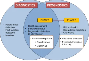
Diagrammatically, the fields of diagnostics and prognostics are shown in Figure 1. Prognostics involves two phases, with the first one overlapping with diagnostics: an assessment of the current health status. Severity detection, health assessment, and degradation identification are the terms used for describing this phase in the literature. The second phase, which is the actual prognostics, aims to predict the failure time by forecasting the degradation trend leading to an estimate of RUL. Prognostics implies forecasting of the system’s/component’s future health level by propagating the current health level to a failure threshold.
In general, a prognostic model can be categorised into one of four classes: 1) DdM, 2) PbM, 3) Knowledge-based model,
and 4) Hybrid models. Here the emphasis is on classes 1 and 2 and their combination in class 4. The various approaches used in these three classes are now described in this order.
Figure 1. Prognostic and diagnostic phases
DdMs employ routinely collected monitoring data and/or historical event data. They attempt to track the degradation of an asset using extrapolation or projection techniques (e.g. regression, exponential smoothing, or neural networks) or match similar patterns in the history of relevant samples to infer RUL. They also rely on the past patterns of deterioration to forecast future degradation. Usually operational variations, manifest as system or loading inputs, are not involved in data-driven prognostic modelling. An assumption for models in this category is that the future system inputs or operational profile remains constant, or consistent with the past data. Since data-driven prognostics have no engineering information related to the asset or system, they are considered to be black-box operations (Zhang et al., 2009). DdMs are divided into two categories: Statistical models and Artificial Intelligence-Based (i.e. machine learning) models.
Statistical approaches construct models by fitting a probabilistic model to the data without knowledge of any engineering or physical principle. These approaches rely on statistical models and observed data to support the forecasting of the RUL of equipment. A comprehensive study on statistical DdMs for RUL estimation was conducted by (Si et al., 2011). Hidden Markov Model variants (e.g. HMM, HSMM) (Kwan et al., 2003), Wiener and Gamma processes (Wang & Carr, 2010), and Auto-Regressive Moving Average variants (Marjanovic et al., 2011) are examples of statistical DdMs.
Artificial Intelligence (AI), or machine learning, models attempt to recognise complex patterns and make intelligent decisions based on the empirical data. Machine learning approaches are adaptable to situations where problem solutions require knowledge that is difficult to specify, however plentiful data or observations are available. Artificial Neural Networks, Self-Organising Maps, and decision trees are common examples of machine learning
approaches to be used for supporting detection and diagnostics as well as prediction processes (Gebraeel & Lawley, 2008).
Both statistical and machine learning methods employ the degradation patterns of sufficient samples representing equipment failure progression. This requirement is the major challenge in data-driven prognostics since it is often not possible to obtain enough samples of failure progressions. Predominantly, industrial systems are not allowed to run until failure, due to undesired consequences. However, the quality and quantity (sample size) of system monitoring data has a big influence on data-driven methods. Virkler et al. (1979) report that a crack propagation dataset should contain at least fifty samples in order to be considered for meaningful analysis. Sample sizes of prognostic datasets found in the literature range from ten to a hundred (Baruah & Chinnam, 2005). Another challenge for DdMs is the computational complexity of modelling, due to the large number of statistical calculations necessary. In the absence of prior knowledge about the failure mechanism, determining the failure threshold is considered to be another challenge. Similarity-based Prognostics (SBP) is a generic type of DdM based on similarity measures between degradation data collected from other samples and the test specimen signal. The SBP approach is a powerful method for RUL estimation, notably when the historical training sample size is relatively large. In addition, it is suitable for cases where the degradation path is not necessarily exhibiting a monotonic propagation pattern, which is difficult to model using parametric approaches (Wang, 2010). Zio & Di Maio (2010) developed a similarity-based prognostics methodology for estimating the RUL of components in nuclear systems. The presented hybrid model in this paper is based on similarity based prognostics (SBP).
Mahalanobis distance based principal component health index has been used in (Wu et al., 2018). Switching state space model has been proposed in (Peng et al., 2018) to characterize the degradation path.
PbMs involve describing the physics of the failure progression mechanism (Daigle, 2014). In order to provide knowledge rich prognostics output, a PbM attempts to combine defect growth formulas, system specific mechanistic knowledge and monitoring data. These models assume that an accurate mathematical model for degradation can be constructed from first principles. Model parameters may be identified using empirical data obtained from specifically designed experiments (Liao & Kottig, 2014). Particle filters, also called ‘Sequential Monte Carlo Estimators’, have been used widely in prognostics, particularly integrated into physics-based models. Some of the examples found in the literature are: fatigue crack propagation modelling for various engineering structures (Zio & Peloni, 2011), battery capacity modelling (An et al.,
2013), centrifugal pump degradation modelling (Daigle & Goebel, 2013), thermal processing unit degradation (Butler & Ringwood, 2010), pneumatic valve modelling (Daigle & Goebel, 2010), DC-DC converter system level degradation modelling (Samie, 2014), Isolated Gate Bipolar Transistor degradation modelling (Saha et al., 2009), Proton Exchange Membrane Fuel Cells life modelling (Jouin et al., 2014), and Lumen degradation modelling for LED light sources (Fan et al., 2015).
PbMs are considered to be more accurate if an accurate mathematical model representing the degradation process can be found. However, PbMs are component or system specific models which means they cannot be applied to other types of component or system in which the physics of failure mechanism differs. Another disadvantage is that the PbMs are costly compared to other approaches (Heng et al., 2009). A summary of the advantages and disadvantages of the PbM and DdM prognostic approaches is shown in Table 1. A highly detailed comparison of prognostic models from an industrial point of view can be found in (Sikorska et al., 2011). Advantages Disadvantages Ph y sic s-Ba se
d More accurate compared to other approaches
Higher precision
Requires less data
Suitable for creation in design phase
More difficult to model
Sensitive to the design and material properties
Insight of the failure mechanism High cost Da ta -Dr iv en Easier to develop Flexible and adaptable
Suitable to component and system levels
Robust to changes in material or design
Low cost
Need data representing the failure progression
Computational complexity
Difficulty in determining of the failure thresholds Table 1. Comparison of prognostic approaches It has been found difficult to predict the trends of all characteristic parameters by using an individual prognostic approach, since the parameters are diverse in real world cases (Peng et al., 2010). Wang (2010) reports that the examples of successful prognostic applications in complex engineering systems are still scarce. Such complex systems exhibit immensely stochastic and non-linear degradation profiles which make them difficult to model accurately. Therefore, prognostics is considered the Achilles’ heel of condition based maintenance (CBM) and PHM (Vachtsevanos & Valavanis, 2009). Both, DdM and PbM approaches have different requirements in order to capture the degradation process and predict the RUL of a system.
Hybrid prognostic modelling combines multiple prognostic approaches in order to leverage the strengths of individual methods, leading to an enhanced prognostic outcome. Prognostic datasets that can be efficiently employed for a
DdM, as well as for a PbM, are remarkably sparse in the literature (Eker et al., 2012). The datasets either lack sufficient data samples or are missing efficient physical modelling in most cases. Thus, development of a DdM and PbM for the same system and their integration is a great challenge. However, the use of hybrid prognostic techniques is a relatively new area and offers a promising line of research. The hybrid prognostic approach has several advantages, some of which are:
Compensation for the imperfections of individual approaches.
Improvement of prediction accuracy.
Computation complexity due to extensive data processing required in DdM may be reduced with the support physics-based models.
Combining approaches can compensate for lack of data, the main thrust of this paper.
Hybrid prognostic models found in the literature (Liao & Kottig, 2014; Zhang et al., 2006) are application specific and combinations of these models is achieved by using one method for health state estimation and another for the RUL prediction. For instance, Huang et al. (2007) presented a hybrid methodology in which the health state of the system is estimated by a Self-Organising Map baseline, supported by using Minimum Quantisation Error, and RUL prediction is performed by a trained Back Propagation Neural Network. A number of researchers have used a DdM to infer the measurement model, and use a physical model to predict RUL. The measurement model maps the sensory data to the underlying system state, which is not measured. In other words, PbM and DdM approaches are used in different steps of the PHM process, such as health state identification and forecasting (Jardine et al., 2006; Huang et al., 2007; Baraldi et al., 2012; Wang et al., 2018).
There are studies that combine DdM and PbM in the state forecasting process (Liao & Kottig, 2014; Goebel et al., 2006; Goebel et al., 2007). These methods run the DdM and PdM independently and combines their results using fusion techniques such as Dempster-Shafer theory.
In (Zhao et al., 2018), an integrated method has been presented that combines Bayesian update with Archard's wear model. The presented method is unique to the given wear model. There is no hybrid prognostic approach in the literature that integrates a given PbM and DdM approaches in the forecasting process that interact with each other. In other words, the forecast of one affects the forecast of the other. This research aims to contribute to the literature by filling this gap, as well as demonstrating good accuracy with scarce data. In addition, the hybrid model requires the output of the physics based model and can be applied with any physical model.
3.METHODOLOGY
The hybrid method assumes that the current health state has already been identified and focuses only on the forecasting of the health state (failure) progression. The integration of physics based and data-driven method is performed in the forecasting process. Physics based methods are good in forecasting within the short time period whereas data-driven methods may reflect the long term patterns in the forecasting process. The forecasting process is divided in two phases: Short-term Forecasting and Remaining Useful Life (RUL) estimation with long term forecasting. Physics based method performs the short term forecasting first. Then, the last forecasted time point by physics based method is assumed to be the current time by the data-driven method. The forecast by the data driven method starts in the time point after the end of the forecast of the physics based method. In other words, data driven method relies on the forecast of the physics based method. The following subsections discuss each of these phases in detail.
This section is concluded with a subsection stressing on the particle filters.
3.1.Short-term Forecasting
This step is achieved through the physics-based approach. This requires an equation to define the health state progression between the health state at time t-1 and the health state at time t. Hence, the health state at time t can be estimated using the health state at time t-1 in the equation. There are many physical models in the literature for different scenarios representing the failure degradation; crack growth and filter clogging are examples of just two of them. Any physical model with inputs and outputs can be presented as shown in Figure 2.
Figure 2. Input and Outputs of Physical Model Observations affected by the health states and model parameters have been used as input. The forecasted health states have been obtained as an output. Crack growth and filter clogging failures have been selected for demonstration of the presented hybrid model and their physical models are discussed in the next two subsections.
3.1.1.Paris Law for Crack Growth Failure Mode Physics-based modelling of fatigue crack propagation is a widely studied research area. The simplest and most commonly used fatigue crack propagation model is the Paris Law (Paris & Erdogan, 1963). It is shown in Eq. (1), and
expresses the relationship between the crack growth rate per cycle ‘da dN⁄ ’; and the previous crack length ‘a’.
𝑑𝑎
𝑑𝑁= 𝐶(∆𝐾)
𝑚 (1)
𝑑𝑎 : Crack growth
𝑑𝑁 : Cycle change
𝑑𝑁/𝑑𝑁 : Crack growth per cycle
𝐶 : Material Constant
𝑚 : Environment and stress ratio
∆K : Stress intensity factor during cycle Where:
∆𝐾 = ∆𝜎√𝜋𝑎 (2)
𝑎 : Crack length
∆σ : Range of stress amplitude
For sufficiently small ‘ dN ’, the Paris Law can be approximated into a discretised state transition function as follows:
𝑎𝑡= C(∆𝜎√𝜋𝑎𝑡−1 )𝑚𝑒𝑤𝑡𝑑𝑁 + 𝑎𝑡−1 (3)
at : Crack length at time t (dynamic state parameter)
wt : Process noise (wt~N(0, σw2)).
Derivatives of this well-known equation are widely used in the prediction of fatigue life (Liu et al., 2015). Refer (Eker, 2015) for a detailed literature review on crack propagation modelling and estimation approaches.
3.1.2.Filter Clogging
Severity of filter clogging is the main parameter used to identify a replacement time for a filter. Direct measurement of severity may not be possible during the usage of the system and so the aim of the physical model is to calculate the severity of filter clogging using the measured parameters. Pressure drop across the filter, volumetric flow rate, cake thickness, and porosity are the main dynamic parameters revealing the clogging severity of the filter. It may be feasible and easy to measure some of these parameters. If direct measurement is not possible for some of them, some other measures may be used to derive them. The well-known Ergun equation formulates the relationship between pressure drop and the other clogging parameters and is a detailed version of the renowned Kozeny-Carman equation. Tien & Ramarao (2013) claim that the Ergun equation is the most commonly used model capable of describing the pressure drop and flow rate correlation.
A modified version of the Ergun equation (Eker et al., 2016) that incorporates effective filtration area rate (i.e. ‘a’) in the filter is used in this study. Effective filtration area rate, the new parameter in the equation, accommodates the effects of the latest stages of filtration. The modified version of the Ergun equation is given as Eq. (4).
∆P =10AVsμ(1−ϵ)2L
Dp2ϵ3a +
B(1−ϵ)ρVs2L
ϵ3Dpa (4)
∆P : Pressure drop
Vs : Superficial (empty-tower) velocity
μ : Viscosity of the fluid
ϵ : Porosity of the bed (or cake)
L : Total height of the bed (e.g. cake thickness)
ρ : Liquid density
Dp : Diameter of the spherical particle
A, B : Constants
The formula given in Eq. (4) cannot be used for prognostics purposes directly. The dynamic rate of change in the pressure drop will be more useful for prognostics purposes. In other words, a dynamic state transition is required for modelling the degradation behaviour of the system. If the severity of the filter clogging increases, then the pressure drop changes accordingly. Thus, the presented equation is transformed into a dynamic state transition equation to be able to serve for prognostics purposes. The rate of change in pressure drop in a small time (‘dt’) can be formulated as:
∆Pt+dt≅ ∆Pt+ ∆Pt′dt + wt (5)
Eq. (5) represents a nonlinear pressure drop across an incremental step. ′wt ′ in the equation represents the process noise whereas the ‘∆Pt′’ term can be obtained by taking the first derivative of the equation given in Eq. (4):
∆P′=10AVsμ d2aϵ3 [ ϵ(1−ϵ)2L′−(1−ϵ)(3−ϵ)Lϵ′ ϵ + (1−ϵ)2La′ a ] + BρVs2 daϵ3 [ (2ϵ−3)Lϵ′ ϵ + (ϵ−1)La′ a + (1 − ϵ)L ′] (6)
Filter clogging severity is identified based on the pressure drop across the filter. If all the parameters on the right-hand side of the Eq. (6) are known, then the pressure drop can be calculated by adding the pressure drop increase rate to the previous pressure drop value. A Particle Filter (PF) is employed for estimation of the parameters within the state transition function. Refer (Eker, 2015) for a detailed literature review on porous medium clogging modelling and estimation approaches.
3.1.3.Particle Filters
In general, dynamic systems can be modelled in the form of a state transition equation, which describes the evolution of its state through time (Paris & Erdogan, 1963). The system state and measurement models underpinning Particle Filter processes are given in Eq. (7) and (8). A system state model, represented in Eq. (7), formulates the state of a system at time
𝑘 is based on the system state at time 𝑘 − 1; the future progression of the states is estimated based on the current state. In the case studies presented in this paper dynamic filter clogging and crack propagation models are used as state transition equations.
𝑥𝑘= 𝑔𝑘(𝑥𝑘−1, 𝜃𝑘−1, 𝑤𝑘−1) (7)
𝑧𝑘= ℎ𝑘(𝑥𝑘, 𝑣𝑘) (8)
𝑔𝑘: : Dynamic state transition equation
𝑥𝑘, 𝑥𝑘−1: State vectors at discrete time points k and k-1
𝜃𝑘 : Model parameter vector
𝑤𝑘 : Process noise
ℎ𝑘: : Measurement equation
𝑧𝑘 : Measurement at time point k
𝑣𝑘 : Measurement noise
Particles, evolving in the system, can be represented as ‘{𝑥𝑘𝑖, 𝜃𝑘𝑖, 𝑤𝑘𝑖}𝑖=1𝑁 ’, where ‘𝑁’ symbolises the total number of particles and ‘𝑖’ is the particle index. Each particle has a state variable ‘𝑥’, model parameters ‘𝜃’, and a process noise value ‘𝑤’, which evolves through time. This means that the degradation distribution will be constructed with N particles. Generally, the higher number of particles used in the construction of a parameter distribution the better the system is represented. Therefore, a reasonably high number for ‘𝑁’ in the modelling of degradation is selected. However, excessively higher numbers for ‘𝑁’ will increase the computational complexity, which may be burdensome when dealing with higher numbers of system parameters. The model parameters are symbolised in ‘𝜃’ which encapsulates the state transition equation parameters, the state transition equations are based on the physical equations representing the degradation. ‘𝑥’ and ‘𝑧’ are the state variables and measurement values, respectively.
In particle filters, the posterior distribution filtering process usually comprises three recursive steps: 1) Prediction, 2) Update, and 3) Resampling. In the prediction step, the system state is predicted using the previous step’s updated parameters, via the state transition equation. Then the predictions are updated for the current time step by using a likelihood function shown in Eq. (9). Likelihood functions assign weights to particles according to the closeness to the measurement at each time point. In the resampling step, the particles with lower and higher weights are eliminated and duplicated, a process called the inverse CDF (cumulative density function) method (An et al., 2013). This filtering process is called Sequential Importance Resampling (SIR) particle filters. 𝐿(𝑧|𝑥, 𝜃, 𝜎) = 1 √2𝜋𝜎𝑒𝑥𝑝 [ 1 2( 𝑧−𝑥(𝜃) 𝜎 ) 2] (9) 𝜎 : Standard Deviation
The parameter learning process is performed using the data collected until the current time at which point the forecasting will start based on the learned parameters. In the extrapolation phase where the parameter learning has stopped, the state parameter vector (i.e. ‘𝑥’) is projected continuously by using the state transition equation (with the fixed parameter distributions) until it reaches the failure threshold. In this way, ‘𝑁’ trajectories give the distribution of
RUL estimations. The mean or median of the RUL distribution is generally used for visualisation of the estimated RULs. Detailed discussion on the model can be found in (Eker et al., 2016).
3.1.4.Remaining Useful Life Calculation
The RUL calculation is performed using the data-driven approach. The fundamental idea of the RUL calculation in the presented approach is that the asset under observation should degrade in a similar manner to previously degraded assets. In an extreme case, if there exists a perfect match with the health state progression for the asset under observation and one of the previously degraded assets, then the asset is expected to continue degrading the same way as the previously degraded asset has degraded. Thus, one can focus on the RUL of the previously degraded asset rather than forecasting the health state progression of the asset under observation. In general, it is not expected to find a perfect match in health state progressions due to the natural variance between assets. Thus, RUL calculations are based on the weighted sum of RULs of previously degraded assets. The similarity measures of the health state progression of the asset under observation and the health state progression of previously degraded assets are employed instead of weights, as shown in Eq. (10) in RUL calculation.
RUL𝑢t =
∑𝑁𝑖=1(𝑠𝑖RUL𝑡𝑖,𝑠𝑖 )
∑Ni=1𝑠𝑖 (10)
RUL𝑜t : Remaining Useful Life of the asset under observation (o) at time t
𝑁 : Number of previously degraded assets
𝑠𝑖 : Similarity of the health state progressions of the asset under observation and asset i
RUL𝑡𝑠
𝑖 : Remaining useful life of asset i at time 𝑡 𝑠
𝑡𝑖,𝑠 : The time where the most similar segment of health progression of the asset i to the health progression of asset under observation starts Similarity (𝑠𝑖) is used as the main criteria for long term forecasting and is calculated based on the function given in Eq. (11)
𝑠𝑖= e− (dimin)2
λ (11)
λ : Gaussian variable of the similarity function
dimin : Minimum distance of the segments of health progression of asset 𝑖 to the health progression of the asset under observation
The minimum distance measure (dimin) quantifies the distance of the most similar segment of health progression of asset 𝑖 (zi) to the health progression of the asset under observation (z0). The middle health state progression with the star sign at the current time in Figure 3 represents the health progression of the asset under observation (z0), whereas the
two solid line progressions on the sides of z0reaching to the threshold represent the health state degradation of previously degraded assets (z1, z2). The health progression of the asset under observation ( z0 ) includes two segments: past progression and short-term forecasted progression. Past progression (‘n0’ segment) represents the recent past health state progression until the current time (zt−𝑛𝑜,…,t
o ). The second segment (‘n1’ segment) is the forecasted health state progression obtained in short term forecasting (zt,…,t+𝑛1
o ),
which is obtained from PbM. Star sign in the health progression of the asset under observation (z0) shows the current time. Thicker lines on the left and right sides of the current time (star sign) in z0 represent the n0 and n1 segments, respectively.
The similarity calculation for the data-driven approach is based on both of these segments: recent past health progression and short term forecasted health progression. The forecasted values bring the failure point closer, which is expected to increase the estimation accuracy. The time series data of health state progression of the asset under observation includes a total of T = n0+ n1+ 1 data points. The accuracy of the physics-based model, selection of the number of forecasted points (n1) and the number of past data to be used (n0) are the elements affecting the hybrid performance; their effect on the results is explored later, in Section IV.
The second time series data in the similarity calculation is the health state progression of one of the previously degraded assets (zi). The previously degraded assets are expected to include full health state failure progression from brand new to failure. Since the length of the time series of z0 is less than the length of the time series of zi (zt−𝑛o 0,…,t+𝑛1 vs z1,2,…,Ki )), multiple parts of the longer time series can be compared with
z0. The shorter time series (z0) can be compared to the longer time series (with zi) and similarities calculated. The part of the health progression of asset i that is most similar to
zt−𝑛0,…,t+𝑛1
o will be used to quantify the similarity of the asset i.
The basic time series similarity calculation requires an equal number of data points from both time series. There are complex methodologies to calculate the distance between two time series data with different number of data points such as dynamic time warping. The presented approach is based on the similarity calculation of time series data with the same number of points in order not to increase the computational complexity. The most similar segment within the health state progression of previously degraded asset i is defined as the similarity of the health state progression of the asset under observation (zt−𝑛0,…,t+𝑛1
o ) and the health state progression of previously degraded asset i as shown in Eq. (12). The equation checks different length of segments as well as different data starting points for the segments.
dimin= min(𝑑1,𝑇𝑖 , 𝑑2,𝑇𝑖 , … , 𝑑𝛼,𝑇𝑖 , … , 𝑑𝑓−𝑇𝑚𝑖𝑛,𝑇𝑚𝑖𝑛 𝑖 ) (12)
𝑑𝛼,𝑇𝑖 : Distance of health progression of the asset under
observation to the health progression segment starting from data point 𝛼 with of 𝑇 number of data points from asset i 𝑇 : Number of data points in the health progression of asset
under observation, T = n0+ n1+ 1
𝑇𝑚𝑖𝑛 : Minimum length of time series data to be used in similarity calculation
The distance calculation between two segments with the same length is given in Eq. (13).
𝑑𝛼,𝑇𝑖 = √∑ ‖z α+ji − zt−𝑛0+j o ‖2 𝑛0 j=0 + ∑ ‖zα+𝑛0+k i − z t+ko ‖ 2 𝑛1 k=1 (13)
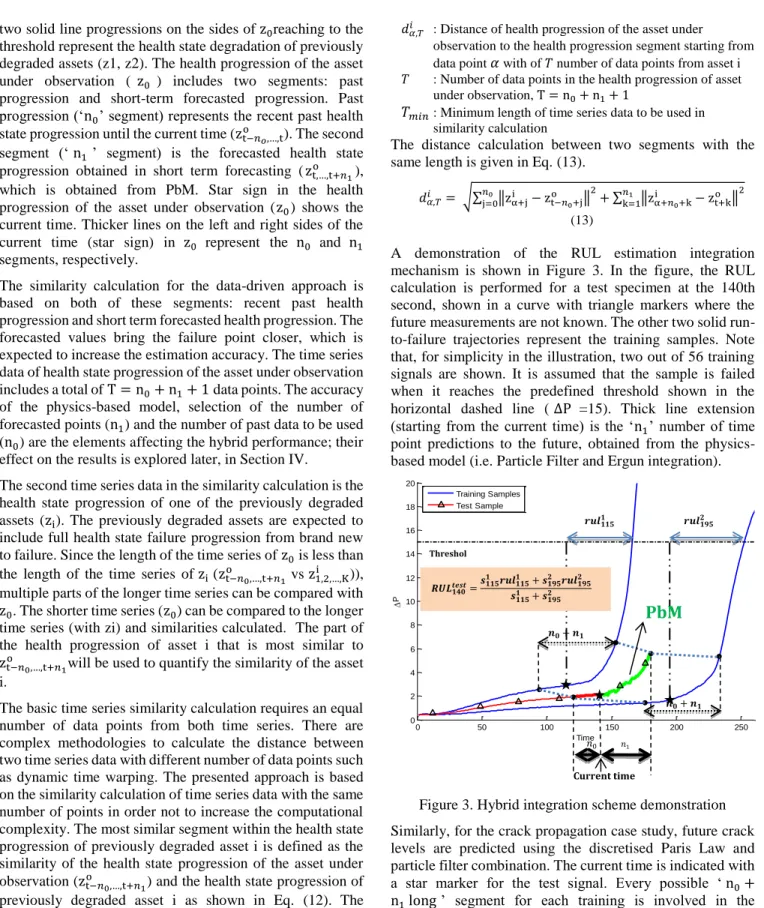
A demonstration of the RUL estimation integration mechanism is shown in Figure 3. In the figure, the RUL calculation is performed for a test specimen at the 140th second, shown in a curve with triangle markers where the future measurements are not known. The other two solid run-to-failure trajectories represent the training samples. Note that, for simplicity in the illustration, two out of 56 training signals are shown. It is assumed that the sample is failed when it reaches the predefined threshold shown in the horizontal dashed line (∆P =15). Thick line extension (starting from the current time) is the ‘n1’ number of time point predictions to the future, obtained from the physics-based model (i.e. Particle Filter and Ergun integration).
Figure 3. Hybrid integration scheme demonstration Similarly, for the crack propagation case study, future crack levels are predicted using the discretised Paris Law and particle filter combination. The current time is indicated with a star marker for the test signal. Every possible ‘n0+
n1 long’ segment for each training is involved in the similarity calculation and similarity values are assigned to each segment. The most similar segment for each training segment is detected and it’s RUL and similarity values are used in the final RUL calculation demonstrated in Figure 3.
𝒏
𝟎 0 50 100 150 200 250 0 2 4 6 8 10 12 14 16 18 20 Time P Training Samples Test Sample Current time 𝑛0 𝑛1 𝒓𝒖𝒍𝟏𝟏𝟓𝟏 𝒏𝟎+ 𝒏𝟏 𝒓𝒖𝒍𝟏𝟗𝟓𝟐 Threshol d 𝒏𝟎+ 𝒏𝟏PbM
pre
𝑹𝑼𝑳𝟏𝟒𝟎𝒕𝒆𝒔𝒕=𝒔𝟏𝟏𝟓𝟏 𝒓𝒖𝒍𝟏𝟏𝟓𝟏 + 𝒔𝟏𝟗𝟓𝟐 𝒓𝒖𝒍𝟏𝟗𝟓𝟐 𝒔𝟏𝟏𝟓𝟏 + 𝒔 𝟏𝟗𝟓 𝟐For instance, ‘s1151 ’ and ‘rul1151 ’ represents the similarity and RUL values of the most similar segment for training sample one. This means that the first training sample’s 115th second reference point is the most similar point to the current time of test specimen. Similarly, for the second training specimen, the 195th second time point stands out as having the highest similarity.
The presented hybrid approach conjoins the future estimations in the similarity calculation, which is anticipated to enhance the prognostic results compared to the distinct usage of physics-based or data-driven approaches. The results of this hybrid approach are discussed in the next section.
4.RESULTS AND DISCUSSION
4.1.Scenarios
In each of the two use cases, the integration of the DdM and the PbM approaches is analysed in five different scenarios. The first two scenarios represent the case of using only one of the models (PbM, DdM) assuming that all of the requirements (statistically sufficient available degradation data, sufficient knowledge about the physics of the failure, etc.) have been met. For the remaining three scenarios, the DdM and PbM approaches are combined in the hybrid model described in Section III, but fed with limited amounts of data to observe how the hybrid method performs. In scenarios three and four both models are used, but only the requirements of one of the models is fully met. The other model is degraded, as explained in detail below. Lastly, the fifth scenario represents a real-world prognostic application case where both models are supplied with limited data. In the third scenario, the data-driven model (DdM) is identical to the second case whereas the physics-based model is weakened on purpose to observe the compensation effects on the hybrid results. The physics-based model is crippled by starting with poor initial parameters for the particle filter modelling. These modifications are anticipated to result in a weakened prognostic capability of the physics-based model. Similarly, in the fourth scenario, the DdM is weakened by reducing the number of training samples. Training samples are the historical run-to-failure data observations to be used in the training of the data-driven model. Reducing the data implies insufficient training of the model, resulting in poor prognostic results.
The first four scenarios assume that the requirements of one of the models have been fully met. In other words, they are representative of the conditions where the data sources feeding the data or physical model are exceptionally rich to provide remarkably precise prognostic outputs. However, it is often difficult to model system/component degradation profiles completely due to many reasons which have already been discussed. Therefore, these perfect modelling cases are
here labelled as unrealistic. The fifth scenario is, by contrast, realistic.
The RUL estimation results obtained under these scenarios are compared based on Prognostic Horizon (PH), 𝛼 − 𝜆
performance, Relative Accuracy (RA), and Convergence metrics (Saxena et al., 2008). PH is defined as the range in between the point where the predictions fall under the allowable error bound (defined by 𝛼) for the first time and the end-of-life time point. The 𝛼 − 𝜆 performance metric determines whether the predictions fall within the shrinking accuracy cone (defined by 𝛼) around the actual RUL values. The output of the metric is binary. However, it can be converted to percentage values if the metric is implemented at multiple time instances. RA is similar to the 𝛼 − 𝜆
accuracy measure. Instead of inspecting whether the predictions fall within the boundaries, cumulative relative accuracy (CRA), the weighted average of the RA values for the time instances of prediction points, is used. Convergence is the final metric to be verified in the hierarchical design. The following subsections present the results for the two applications.
4.2.Crack Propagation Modelling
The Virkler dataset consists of 68 crack growth trajectories collected under well-controlled fatigue loading experiments. The experiments were conducted under constant amplitude fatigue loading and controlled environmental conditions. Several preliminary tests were conducted for determining the actual load levels for the material type. The specimens aged in the experiments were 2024-T3 aluminium alloy plates which were drilled in the centre to form a 2.54mm initial notch.
During the aging process, samples were subjected to cyclic tensile loading at 𝑅 = 0.2 stress ratio with ∆𝜎 = 48.28 𝑀𝑃𝑎
stress range levels. Throughout the experiments, cycle numbers were recorded at fixed increments in crack lengths (i.e. ∆𝑎 = 0.2𝑚𝑚) until the crack reached its predefined final length of 49.8mm. Note that in the final stages of data collection, cycles were recorded at 0.4mm and 0.8mm increment levels as well. Each signal in the dataset contains 164 measurement points throughout its degradation path. Table 2 gives the details of the scenarios for the crack growth dataset.
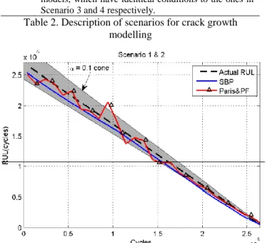
A visualised comparison of the first two scenarios (i.e. physics-based and data-driven model) is depicted in Figure 4. The x-axis is the life period of the specific sample, whereas the y-axis stands for the corresponding RUL values. In this figure, the dashed linear line represents the actual RUL values. Actual RUL values for a specimen are calculated by subtracting the current cycle from the End of Life (EoL) value specific to the specimen. The small alpha cone gives visual confirmation of the accuracy of the rich models; the results from a single test specimen show that both models
stay within a 10% error bound predominantly throughout the degradation process.
Scen arios
Details
1 Physics based model for crack propagation with a rich data source and optimised initial model parameters. 2 59 out of 68 samples (i.e. ~85%) are selected to be used
in the training of the modified SBP model while the remaining nine samples (i.e. ~15%) are left for testing the algorithm.
3 The physics-based crack propagation model is crippled by initialising the model parameters poorly. The data-driven model has identical conditions to that in Scenario 2.
4 In order to limit the capabilities of the data-driven model, the number of training samples is significantly reduced (i.e. training sample size is dropped to 7). The physics-based model has identical conditions to the one in Scenario 1.
5 Poor conditions for both physics-based and data-driven models, which have identical conditions to the ones in Scenario 3 and 4 respectively.
Table 2. Description of scenarios for crack growth modelling
Figure 4. PbM vs DdM RUL visualisation on a crack growth sample
Table 3 gives the prognostic evaluation results for all scenarios. PbM(c) and DdM(c) indicate complete model results with all requirements satisfied. Prognostic evaluation metrics PH, 𝛼 − 𝜆 performance, CRA, convergence, normalised root mean squared error (nRMSE) results are given in the table. nRMSE metric results are obtained by normalising the RMSE results with mean lives (run-to-failure) in the relevant conditions. The results highlighted in bold in the tables indicate the highest performance for scenarios in which the hybrid scheme is used.
As shown in Figure 4 and illustrated by all the various performance metrics in Table 3, both PbM(c) and DdM(c) results are very good when supplied with all the data.
Scenario 1 2 3 PbM(c) DdM(c) PbM Hybrid PH (%) 95.33 93.26 75.47 93.6 𝛼 − 𝜆 (%) 58.16 68.86 12.71 67.13 CRA (%) 85.99 88.42 61.64 88.85 Convergence 0.55 0.53 0.57 0.52 nRMSE (%) 5.97 4.63 22.46 4.47 Scenario 4 5 DdM Hybrid PbM DdM Hybrid PH (%) 29.22 52.04 76.63 21.19 89.95 𝛼 − 𝜆 (%) 5.9 15.19 11.28 6.25 18.63 CRA (%) 60.36 72.14 61.26 56.03 65.18 Convergence 0.73 0.65 0.59 1.16 1.02 nRMSE (%) 15.43 13.07 23.09 16.56 13.3 Table 3. Performance metrics comparison for crack
propagation case study
Comparing scenarios one and four, the complete PbM (scenario 1) and its hybrid use with a degraded DdM (scenario 4), the PbM is expected to perform best and indeed does. On the other hand, for scenarios two and three, the complete DdM (scenario 2) and its combination with a degraded PbM (scenario 3), the complete model DdM was expected to perform the highest. However, the hybrid model produced very close results to the mature DdM model, with some parameters showing even better results. It was because the integration scheme is based on the similarity-based data-driven model. Hence, the PbM future estimations add value rather than corrupt the model. Integrating these future estimations do not enhance the immature SBP model. The fifth scenario is the reason for developing the hybrid scheme, since it is considered as the real-life prognostic scenario, where both PbM and DdM are immature. If one further investigates the tables for both cases, the hybrid model outperforms the other methods for nine out of ten metrics. This indicates that the integration mechanism enhances prognostic capability in general. Also, the results show that using an individual deteriorated model will not produce robust outputs. The data-driven model produces roughly 20% prognostic horizon levels for the crack propagation case. However, the integration scheme brings robustness, where the PH percentage level rises to nearly 90%, a good deal beyond the deteriorated PbM value of 77%. To conclude, one of the main goals for this research was to develop a generic integration scheme to be used in hybrid modelling, in which incomplete data-driven and physics-based models were integrated. The results obtained from this case study shows unequivocally that the hybrid scheme produces significantly better prognostic results than either of the prognostic schemes on their own.
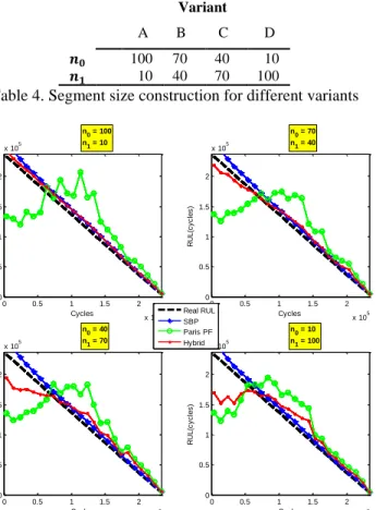
To further examine the bias between DdM and PbM, Scenario 3 is selected. Referring to Figure 3, ‘𝑛0’ and ‘𝑛1’ can be used as the bias between DdM and PbM. For instance, increasing ‘𝑛0’ means involving more data points from the past into the similarity calculations, which implies the hybrid integration system is biased towards the DdM. Contrarily, where the system is more biased to PbM, the ‘𝑛1⁄𝑛0’ ratio will increase. The use of ‘𝑛0’ and ‘𝑛1’ for the variants chosen is summarised in Table 4.
Variant A B C D 𝒏𝟎 100 70 40 10 𝒏𝟏 10 40 70 100
Table 4. Segment size construction for different variants
Figure 5. System bias comparison
Figure 5 shows the effect of these variations. The top left plot in the figure represents the highest bias towards the DdM, with an ‘𝑛0⁄𝑛1= 10’ bias rate. The rate decreases moving through to the bottom right where it is 0.1. Note that, as the DdM is complete and the PbM is incomplete, Scenario 3 being chosen, the degeneration in the hybrid model results is apparent as the bias towards PbM is made. The hybrid curves remain significantly closer to actual RUL values when the bias is directed to the complete DdM model. This integration mechanism gives users the flexibility to tune the bias values as desired.
4.3.Filter Clogging Modelling
The second case study concerns filter clogging. This dataset consists of fifty-six run-to-failure samples obtained from well-controlled accelerated filter clogging experiments (Eker
et al., 2016). Table 5 gives the details of the prognostic scenarios for the filter clogging failure mode.
Scenarios Details
1 Physics-based model for filter clogging with a rich data source and optimised initial model parameters. 2 40 out of 56 samples are selected to be used in the training of the modified SBP model while the remaining sixteen samples are left for testing the algorithm.
3 The physics-based model is crippled by starting with poor initial parameters used in the particle filter modelling. The cake thickness simulation is also weakened by adding randomly shifted errors. 4 In order to limit the capabilities of the data-driven
model, the number of training samples is significantly reduced (i.e. training sample size is dropped to 5).
5 Poor conditions for both physics-based and data-driven models which have identical conditions to the ones in Scenario 4 and 5 respectively.
Table 5. Description of scenarios for filter clogging Table 6 organises all the prognostic evaluation results for the five scenarios. PbM(c) and DdM(c) column names indicate that the model is complete, where they belong to scenarios one and two respectively.
Scenario 1 2 3 PbM(c) DdM(c) PbM Hybrid PH (%) 96.22 91.51 60.13 93.02 𝛼 − 𝜆 (%) 59.65 27.25 16.61 27.16 CRA (%) 83.56 72.85 62.58 72.80 Convergence 0.51 0.51 0.55 0.51 nRMSE (%) 7.17 11.09 26.24 11.20 Scenario 4 5 DdM Hybrid PbM DdM Hybrid PH (%) 80.70 90.11 55.70 75.85 84.97 𝛼 − 𝜆 (%) 13.50 42.09 4.68 14.18 19.15 CRA (%) 61.47 81.34 63.25 59.62 70.24 Convergence 0.53 0.51 0.53 0.63 0.52 nRMSE (%) 25.04 10.58 20.30 26.04 17.60 Table 6. Performance metrics comparison for filter clogging
case study
From Table 6, both PbM(c) and DdM(c) results are very good when supplied with all the data. The hybrid schemes are again seen to be noticeably better than the degraded method, i.e. in scenario 4 the hybrid is much better than the degraded DdM. The hybrid method is compensating for the lack of data by combining both techniques.
Comparing scenarios 1 and 3, the performance of the PbM drops significantly but is almost completely recovered by the using the DdM(c) in the hybrid. Scenarios 2 and 4 show a similar story when the DdM(c) results are degraded by using
0 0.5 1 1.5 2 x 10⁵ 0 0.5 1 1.5 2 x 10⁵ Cycles R U L (c y c le s ) n0 = 100 n1 = 10 0 0.5 1 1.5 2 x 10⁵ 0 0.5 1 1.5 2 x 10⁵ Cycles R U L (c y c le s ) n0 = 70 n1 = 40 0 0.5 1 1.5 2 x 10⁵ 0 0.5 1 1.5 2 x 10⁵ Cycles R U L (c y c le s ) n0 = 40 n1 = 70 0 0.5 1 1.5 2 x 10⁵ 0 0.5 1 1.5 2 x 10⁵ Cycles R U L (c y c le s ) n0 = 10 n1 = 100 Real RUL SBP Paris PF Hybrid
very much less data, only 5 samples rather than 40. Again, the hybrid method improves the results in all metrics. Finally, for scenario 5, the hybrid result is the best across all metrics, supplementing the good performance of the DdM with very little data.
To conclude, one of the main goals for this research was to develop a generic integration scheme to be used in hybrid modelling, in which incomplete data-driven and physics-based models are integrated. The results obtained from two engineering case studies verify that the integration scheme produces better prognostic results compared to the particular models which contribute to the hybrid mechanism. Therefore, this integration scheme is anticipated to be applied to other engineering cases to enhance the accuracy of the estimations.
5.CONCLUSIONS
Prognostics is the key component of PHM technologies, which generally involves system monitoring, fault detection and diagnostics, failure prognostics and operating management. Physics-based and data-driven approaches are two of the most commonly used prognostic models in the industry / academia, both approaches having their own strengths and weaknesses. This paper presents a hybrid prognostic model that leverages the strengths of both approaches whilst avoiding the weaknesses where possible. The similarity based prognostics have been modified to include the short-term forecast obtained from physics-based prognostics. The method has been applied on crack growth and filter clogging test cases. The RUL estimations based on the hybrid method are presented and compared with individual physics-based and data-driven approaches. It is concluded that, for real world problems with a shortage of run to failure data, the hybrid approach is much better than either of its constituent techniques.
ACKNOWLEDGEMENT
This research was supported by the IVHM Centre, Cranfield University, UK and its industrial partners.
REFERENCES
An, D., Choi, J. and Kim, N. H. (2013), "Prognostics 101: A tutorial for particle filter-based prognostics algorithm using Matlab", Reliability Engineering & System Safety, vol. 115, no. 0, pp. 161-169.
Baraldi, P., Compare, M., Sauco, S. and Zio, E. (2012), "Fatigue Crack Growth Prognostics by Particle Filtering and Ensemble Neural Networks", 1st european conference of the prognostics and health management society 2012, Vol. 3, 2012, Dresden, Germany, PHM Society, Dresden, Germany.
Baruah, P. and Chinnam, R. B. (2005), "HMMs for diagnostics and prognostics in machining processes",
International Journal of Production Research, vol. 43, no. 6, pp. 1275-1293.
Butler, S. and Ringwood, J. (2010), "Particle filters for remaining useful life estimation of abatement equipment used in semiconductor manufacturing", Control and Fault-Tolerant Systems (SysTol), 2010 Conference on, pp. 436.
Cadini, F., Zio, E. and Avram, D. (2009), "Monte Carlo-based filtering for fatigue crack growth estimation", Probabilistic Engineering Mechanics, vol. 24, no. 3, pp. 367-373.
Daigle, M. and Goebel, K. (2010), "Model-based prognostics under limited sensing", IEEE Aerospace Conference Proceedings, .
Daigle, M. J. and Goebel, K. (2013), "Model-Based Prognostics With Concurrent Damage Progression Processes", Systems, Man, and Cybernetics: Systems, IEEE Transactions on, vol. 43, no. 3, pp. 535-546. Daigle, M., (2014), Model based prognostics (Tutorial),
PHM Society.
Eker O. F. (2015), A Hybrid Prognostic Methodology and its Application to Well-Controlled Engineering Systems (PhD thesis), Cranfield University.
Eker O. F., Camci F., and Jennions I. K., Major Challenges in Prognostics: Study on Benchmarking Prognostics Datasets, PHM Conference Europe, Dresden Germany, July 2012
Eker O.F., Camci F., Jennions I.K. (2016), Physics-based prognostic modelling of filter clogging phenomena, Mechanical Systems and Signal Processing, Volume 75,
15, Pages 395-412, ISSN 0888-3270,
http://dx.doi.org/10.1016/j.ymssp.2015.12.011.
Fan, J., Yung, K. and Pecht, M. (2015), "Predicting long-term lumen maintenance life of LED light sources using a particle filter-based prognostic approach", Expert Systems with Applications, vol. 42, no. 5, pp. 2411-2420.
Gebraeel, N. Z. and Lawley, M. A. (2008), "A neural network degradation model for computing and updating residual life distributions", IEEE Transactions on Automation Science and Engineering, vol. 5, no. 1, pp. 154-163. Goebel K., N. Eklund, and P. Bonanni (2006), “Fusing
competing prediction algorithms for prognostics,” in Proc. IEEE Aerospace Conf., 2006, p.10.
Goebel K., N. Eklund, and P. Bonanni (2007), Prognostic Fusion for Uncertainty Reduction. Wright-Patterson AFB, OH, USA: Defense Technical, 2007
Hecht, H. (2006), "Why prognostics for avionics?", IEEE Aerospace Conference Proceedings, Vol. 2006. Heng, A., Zhang, S., Tan, A. C. C. and Mathew, J. (2009),
"Rotating machinery prognostics: State of the art, challenges and opportunities", Mechanical Systems and Signal Processing, vol. 23, no. 3, pp. 724-739.
Huang, R., Xi, L., Li, X., Richard Liu, C., Qiu, H. and Lee, J. (2007), "Residual life predictions for ball bearings based on self-organizing map and back propagation neural
network methods", Mechanical Systems and Signal Processing, vol. 21, no. 1, pp. 193-207.
Huang, R., Xi, L., Li, X., Richard Liu, C., Qiu, H. and Lee, J. (2007), "Residual life predictions for ball bearings based on self-organizing map and back propagation neural network methods", Mechanical Systems and Signal Processing, vol. 21, no. 1, pp. 193-207.
Jardine, A. K. S., Lin, D. and Banjevic, D. (2006), "A review on machinery diagnostics and prognostics implementing condition-based maintenance", Mechanical Systems and Signal Processing, vol. 20, no. 7, pp. 1483-1510. Jouin, M., Gouriveau, R., Hissel, D., Péra, M. and Zerhouni,
N. (2014), "Prognostics of PEM fuel cell in a particle filtering framework", International Journal of Hydrogen Energy, vol. 39, no. 1, pp. 481-494.
Kothamasu, R., Huang, S. H. and Verduin, W. H. (2006), "System health monitoring and prognostics - A review of current paradigms and practices", International Journal of Advanced Manufacturing Technology, vol. 28, no. 9, pp. 1012-1024.
Kwan, C., Zhang, X., Xu, R. and Haynes, L. (2003), "A novel approach to fault diagnostics and prognostics", Proceedings - IEEE International Conference on Robotics and Automation, Vol. 1, pp. 604.
Liao, L. and Kottig, F. (2014), "Review of Hybrid Prognostics Approaches for Remaining Useful Life Prediction of Engineered Systems, and an Application to Battery Life Prediction", Reliability, IEEE Transactions on, vol. 63, no. 1, pp. 191-207.
Liu, H., Shang, D., Liu, J. and Guo, Z. (2015), "Fatigue life prediction based on crack closure for 6156 Al-alloy laser welded joints under variable amplitude loading", International Journal of Fatigue, vol. 72, no. 0, pp. 11-18.
Marjanovic, A., Kvascev, G., Tadic, P. and Djurovic, Z. (2011), "Applications of predictive maintenance techniques in industrial systems", Serbian Journal of Electrical Engineering, vol. 8, no. 3, pp. 263-279. Paris, P. C. and Erdogan, F. (1963), "A critical analysis of
crack propagation laws", Journal of Basic Engineering, Trans. ASME, vol. Ser. D, no. 85, pp. 528-534. Peng, Y., Dong, M. and Zuo, M. J. (2010), "Current status of
machine prognostics in condition-based maintenance: A review", International Journal of Advanced Manufacturing Technology, vol. 50, no. 1-4, pp. 297-313.
Peng, Y., Y. Wang and Y. Zi, (2018) "Switching state-space degradation model with recursive filter/smoother for prognostics of remaining useful life," in IEEE Transactions on Industrial Informatics, vol. PP, no. 99, pp. 1-1.
Saha, B., Celaya, J. R., Wysocki, P. F. and Goebel, K. F. (2009), "Towards prognostics for electronics components", Aerospace conference, 2009 IEEE, pp. 1. Samie, M., Perinpanayagam, S., Alghassi, A., Motlagh, A. and Kapetanios, E., (2014), Developing Prognostic
Models Using Duality Principles for DC-to-DC Converters.
Saxena, A., Celaya, J., Balaban, E., Goebel, K., Saha, B., Saha, S. and Schwabacher, M. (2008), "Metrics for evaluating performance of prognostic techniques", 2008 International Conference on Prognostics and Health Management, PHM 2008,
Si, X., Wang, W., Hu, C. and Zhou, D. (2011), "Remaining useful life estimation - A review on the statistical data driven approaches", European Journal of Operational Research, vol. 213, no. 1, pp. 1-14.
Sikorska, J. Z., Hodkiewicz, M. and Ma, L. (2011), "Prognostic modelling options for remaining useful life estimation by industry", Mechanical Systems and Signal Processing, vol. 25, no. 5, pp. 1803-1836.
Tien, C. and Ramarao, B. V. (2013), "Can filter cake porosity be estimated based on the Kozeny-Carman equation?", Powder Technology, vol. 237, pp. 233-240.
Vachtsevanos, G. J. and Valavanis, K. P. (2009), Applications of Intelligent Control to Engineering Systems: In Honour of Dr. G. J. Vachtsevanos, Springer. Virkler, D. A., Hillberry, B. M. and Goel, P. K. (1979), "The
Statistical Nature of Fatigue Crack Propagation", vol. 101, no. 2, pp. 148-153.
Wang D., K. Tsui and Q. Miao (2018), "Prognostics and Health Management: A Review of Vibration Based Bearing and Gear Health Indicators," in IEEE Access, vol. 6, pp. 665-676, 2018
Wang, T. (2010), Trajectory Similarity Based Prediction for Remaining Useful Life Estimation (PhD thesis), University Of Cincinnati
Wang, W. and Carr, M. (2010), "An adapted Brownion motion model for plant residual life prediction", 2010 Prognostics and System Health Management Conference, PHM '10, .
Wu J., C. Wu, S. Cao, S. W. Or, C. Deng and X. Shao, (2018) "Degradation Data-Driven Time-To-Failure Prognostics Approach for Rolling Element Bearings in Electrical Machines," in IEEE Transactions on Industrial Electronics, vol. PP, no. 99, pp. 1-1.
Zhang, H., Kang, R. and Pecht, M. (2009), "A hybrid prognostics and health management approach for condition-based maintenance", IEEM 2009 - IEEE International Conference on Industrial Engineering and Engineering Management, pp. 1165.
Zhang, L., Li, X. and Yu, J. (2006), "A review of fault prognostics in condition based maintenance", Proceedings of SPIE - The International Society for Optical Engineering, Vol. 6357 II, .
Zhao F., Z. Tian, X. Liang and M. Xie (2018), "An Integrated Prognostics Method for Failure Time Prediction of Gears Subject to the Surface Wear Failure Mode," in IEEE Transactions on Reliability, vol. 67, no. 1, pp. 316-327. Zio, E. and Di Maio, F. (2010), "A data-driven fuzzy
approach for predicting the remaining useful life in dynamic failure scenarios of a nuclear system",
Reliability Engineering & System Safety, vol. 95, no. 1, pp. 49-57.
Zio, E. and Peloni, G. (2011), "Particle filtering prognostic estimation of the remaining useful life of nonlinear components", Reliability Engineering & System Safety, vol. 96, no. 3, pp. 403-409.
BIOGRAPHIES
Omer Faruk Eker is a data scientist, works as the product and business development manager at Artesis Technology Systems, based in Gebze Technology Park, Turkey. He previously worked as a post-doctorate research fellow at Integrated Vehicle Health Management (IVHM) Centre, involving in a project on physical network modelling of environmental control system of a specific passenger aircraft. He holds his PhD from the School of Aerospace, Transport and Manufacturing, Cranfield University, UK. He received his BS in Mathematics and MS in Computer Science. He was involved in various projects funded by British and Turkish Governments and industrial bodies in between 2009 - 2016. His research interests include fault diagnostics and prognostics, internet of things, predictive maintenance, pattern recognition, artificial intelligence, machine learning and data mining.
Fatih Camci’s main research areas include decision support systems, data analytics and machine learning on various engineering platforms, specifically Prognostics and Health Management. He has BS and MS degrees in Computer Engineering in Turkey and a PhD in Industrial Engineering at Wayne State University, US. He has worked on research projects in the USA, Turkey, UK, and France. He currently works as manager of IT Architecture at AMD, US.
Ian K. Jennions is the director of the IVHM Centre at Cranfield University, UK. He has over 30 years of industrial experience working in engineering and service. He has a Mechanical Engineering degree and a PhD, both from Imperial College, London. He moved to Cranfield in 2008 as Professor and Director of the newly formed IVHM Centre, and has led the development and growth of the Centre, in research and education. Ian is on the editorial Board for the International Journal of Condition Monitoring, a Director of the PHM Society, vice-chair of the SAE IVHM Steering Group and contributing member of the
HM1 IVHM committee, a Chartered Engineer and a Fellow of IMechE, RAeS and ASME. He is the editor of five recent SAE books on IVHM and a co-author of the book: ‘No Fault Found – The Search for the Root Cause’