The ade4 package - I : One-table methods

The ade4 package - I : One-table methods

Introduction

This paper is a short summary of the main classes defined in the ade4 package for one table analysis methods (e.g., principal component analysis). Other papers will detail the classes defined in ade4 for two-tables coupling methods (such as canonical corre-spondence analysis, redundancy analysis, and co-inertia analysis), for methods dealing with K-tables analysis (i.e., three-ways tables), and for graphical methods.

This package is a complete rewrite of the ADE4 software (Thioulouse et al.(1997), http://pbil.univ-lyon1.fr/ADE-4/) for the R environment. It contains Data Analysis functions to analyse Ecological and Environmental data in the framework ofEuclidean Exploratory methods, hence the nameade4(i.e., 4 is not a version number but means that there are four E in the acronym).

The ade4 package is available in CRAN, but it can also be used directly online, thanks to the Rweb system (http://pbil.univ-lyon1.fr/Rweb/). This possibility is being used to provide multivariate analysis services in the field of bioinformatics, par-ticularly for sequence and genome structure analysis at the PBIL (http://pbil.univ-lyon1.fr/). An ex-ample of these services is the automated analysis of the codon usage of a set of DNA sequences by corre-spondence analysis (http://pbil.univ-lyon1.fr/ mva/coa.php).

The duality diagram class

The basic tool in ade4 is the duality diagram Es-coufier(1987). A duality diagram is simply a list that contains a triplet (X,Q,D):

-Xis a table withnrows andpcolumns, consid-ered asppoints inRn(column vectors) ornpoints in Rp(row vectors).

- Q is a p×p diagonal matrix containing the weights of thepcolumns of X, and used as a scalar product inRp(Qis stored under the form of a vector

of lengthp).

- D is a n×n diagonal matrix containing the weights of thenrows ofX, and used as a scalar prod-uct in Rn (Dis stored under the form of a vector of

lengthn).

For example, ifXis a table containing normalized quantitative variables, ifQ is the identity matrixIp

and ifDis equal to 1_nIn, the triplet corresponds to a

principal component analysis on correlation matrix (normed PCA). Each basic method corresponds to a particular triplet (see table 1), but more complex methods can also be represented by their duality di-agram.

Functions Analyses Notes

dudi.pca principal component 1

dudi.coa correspondence 2

dudi.acm multiple correspondence 3 dudi.fca fuzzy correspondence 4 dudi.mix analysis of a mixture of

numeric and factors

5 dudi.nsc non symmetric

corre-spondence

6 dudi.dec decentered

correspon-dence

7 The dudi functions. 1: Principal component analysis, same as prcomp/princomp. 2: Correspondence analysis Greenacre (1984). 3: Multiple correspondence analysis Tenenhaus and Young(1985). 4: Fuzzy correspondence analysisChevenet et al.(1994). 5: Analysis of a mixture of numeric variables and factors Hill and Smith(1976), Kiers(1994). 6: Non symmetric correspondence analysis Kroonenberg and Lombardo(1999). 7: Decentered corre-spondence analysisDolédec et al.(1995).

The singular value decomposition of a triplet gives principal axes, principal components, and row and column coordinates, which are added to the triplet for later use.

We can use for example a well-known dataset from the base package :

> data(USArrests)

> pca1 <- dudi.pca(USArrests,scannf=FALSE,nf=3)

scannf = FALSEmeans that the number of

prin-cipal components that will be used to compute row and column coordinates should not be asked interac-tively to the user, but taken as the value of argument

nf(by default, nf= 2). Other parameters allow to choose between centered, normed or raw PCA (de-fault is centered and normed), and to set arbitrary row and column weights. The pca1object is a du-ality diagram, i.e., a list made of several vectors and dataframes:

> pca1

Duality diagramm class: pca dudi

$call: dudi.pca(df = USArrests, scannf = FALSE, nf=3) $nf: 3 axis-components saved

$rank: 4

eigen values: 2.48 0.9898 0.3566 0.1734 vector length mode content

1 $cw 4 numeric column weights 2 $lw 50 numeric row weights 3 $eig 4 numeric eigen values

data.frame nrow ncol content 1 $tab 50 4 modified array 2 $li 50 3 row coordinates 3 $l1 50 3 row normed scores 4 $co 4 3 column coordinates 5 $c1 4 3 column normed scores other elements: cent norm

pca1$lw and pca1$cw are the row and column

weights that define the duality diagram, together with the data table (pca1$tab). pca1$eig contains the eigenvalues. The row and column coordinates are stored in pca1$li and pca1$co. The variance of these coordinates is equal to the corresponding eigenvalue, and unit variance coordinates are stored

in pca1$l1and pca1$c1(this is usefull to draw

bi-plots).

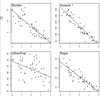
The general optimization theorems of data ysis take particular meanings for each type of anal-ysis, and graphical functions are proposed to draw thecanonical graphs, i.e., the graphical expression cor-responding to the mathematical property of the ob-ject. For example, the normed PCA of a quantita-tive variable table gives a score that maximizes the sum of squared correlations with variables. The PCA canonical graph is therefore a graph showing how the sum of squared correlations is maximized for the variables of the data set. On theUSArrestsexample, we obtain the following graphs:

> score(pca1) > s.corcircle(pca1$co) −2 −1 0 1 2 5 10 15 Murder −2 −1 0 1 2 50 100 150 200 250 300 Assault −2 −1 0 1 2 30 40 50 60 70 80 90 UrbanPop −2 −1 0 1 2 10 20 30 40 Rape

Figure 1: One dimensional canonical graph for a normed PCA. Variables are displayed as a function of row scores, to get a picture of the maximization of the sum of squared correlations.

Murder Assault

UrbanPop

Rape

Figure 2: Two dimensional canonical graph for a normed PCA (correlation circle): the direction and length of ar-rows show the quality of the correlation between variables and between variables and principal components.

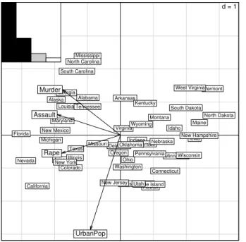
Thescatterfunction draws the biplot of the PCA

(i.e., a graph with both rows and columns superim-posed):

d = 1 Alabama Alaska Arizona Arkansas California Colorado Connecticut Delaware Florida Georgia Hawaii Idaho Illinois Indiana Iowa Kansas Kentucky Louisiana Maine Maryland Massachusetts Michigan Minnesota Mississippi Missouri Montana Nebraska Nevada New Hampshire New Jersey New Mexico New York North Carolina North Dakota Ohio Oklahoma Oregon Pennsylvania Rhode Island South Carolina South Dakota Tennessee Texas Utah Vermont Virginia Washington West Virginia Wisconsin Wyoming Murder Assault UrbanPop Rape

Figure 3: The PCA biplot. Variables are symbolized by arrows and they are superimposed to the individuals dis-play. The scale of the graph is given by a grid, which size is given in the upper right corner. Here, the length of the side of grid squares is equal to one. The eigenvalues bar chart is drawn in the upper left corner, with the two black bars corresponding to the two axes used to draw the bi-plot. Grey bars correspond to axes that were kept in the analysis, but not used to draw the graph.

Separate factor maps can be drawn with the

s.corcircle(see figure 2) ands.labelfunctions:

> s.label(pca1$li) d = 1 Alabama Alaska Arizona Arkansas California Colorado _Connecticut Delaware Florida Georgia Hawaii Idaho Illinois Indiana Iowa Kansas Kentucky Louisiana Maine Maryland Massachusetts Michigan Minnesota Mississippi Missouri Montana Nebraska Nevada New Hampshire New Jersey New Mexico New York North Carolina North Dakota Ohio Oklahoma Oregon Pennsylvania Rhode Island South Carolina South Dakota Tennessee Texas Utah Vermont Virginia Washington West Virginia Wisconsin Wyoming

Figure 4: Individuals factor map in a normed PCA.

Distance matrices

A duality diagram can also come from a distance matrix, if this matrix is Euclidean (i.e., if the dis-tances in the matrix are the disdis-tances between some points in a Euclidean space). The ade4 package contains functions to compute dissimilarity matrices

(dist.binaryfor binary data, anddist.propfor

fre-quency data), test whether they are EuclideanGower

and Legendre (1986), and make them Euclidean

(quasieuclid, lingoes, Lingoes (1971), cailliez,

Cailliez(1983)). These functions are useful to ecol-ogists who use the works ofLegendre and Anderson

(1999) andLegendre and Legendre(1998).

The Yanomama data set (Manly (1991)) con-tains three distance matrices between 19 villages of Yanomama Indians. The dudi.pcofunction can be used to compute a principal coordinates analysis (PCO,Gower (1966)), that gives a Euclidean repre-sentation of the 19 villages. This Euclidean represen-tation allows to compare the geographical, genetic and anthropometric distances.

> data(yanomama)

> gen <- quasieuclid(as.dist(yanomama$gen)) > geo <- quasieuclid(as.dist(yanomama$geo)) > ant <- quasieuclid(as.dist(yanomama$ant)) > geo1 <- dudi.pco(geo, scann = FALSE, nf = 3) > gen1 <- dudi.pco(gen, scann = FALSE, nf = 3) > ant1 <- dudi.pco(ant, scann = FALSE, nf = 3) > par(mfrow=c(2,2)) > scatter(geo1) > scatter(gen1) > scatter(ant1,posi="bottom") d = 100 1 ₂ 3 4 5 7 6 8 9 10 11 12 13 14 15 16 18 17 19 d = 20 1 2 3 4 5 6 7 8 9 10 11 12 13 14 15 16 17 18 19 d = 100 1 2 3 4 5 6 7 8 9 10 11 12 13 14 15 16 17 ₁₈ 19

Figure 5: Comparison of the PCO analysis of the three distance matrices of the Yanomama data set: geographic, genetic and anthropometric distances.

Taking into account groups of

indi-viduals

In sites x species tables, rows correspond to sites, columns correspond to species, and the values are the number of individuals of species j found at site i. These tables can have many columns and can-not be used in a discriminant analysis. In this case, between-class analyses (betweenfunction) are a bet-ter albet-ternative, and they can be used with any duality diagram. The between-class analysis of triplet (X,Q, D) for a given factorfis the analysis of the triplet (G, Q,Dw), whereGis the table of the means of tableX

for the groups defined byf, andDw is the diagonal

matrix of group weights. For example, a between-class correspondence analysis (BCA) is very simply obtained after a correspondence analysis (CA):

> data(meaudret)

> coa1<-dudi.coa(meaudret$fau, scannf = FALSE) > bet1<-between(coa1,meaudret$plan$sta, + scannf=FALSE)

> plot(bet1)

Themeaudret$faudataframe is an ecological

ta-ble with 24 rows corresponding to six sampling sites along a small French stream (the Meaudret). These six sampling sites were sampled four times (spring, summer, winter and autumn), hence the 24 rows. The 13 columns correspond to 13 ephemerotera species. The CA of this data table is done with the

dudi.coafunction, giving thecoa1duality diagram.

The corresponding bewteen-class analysis is done with the betweenfunction, considering the sites as classes (meaudret$plan$sta is a factor defining the classes). Therefore, this is a between-sites analysis, which aim is to discriminate the sites, given the dis-tribution of ephemeroptera species. This gives the

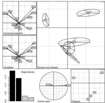
bet1duality diagram, and Figure 6 shows the graph obtained by plotting this object.

d = 1 Canonical weights d = 1 Eda Bsp Brh Bni Bpu Cen Ecd Rhi Hla Hab Par Cae Eig Canonical weights Variables Eda Bsp Brh Bni Bpu Cen Ecd Rhi Hla Hab Par Cae Eig Variables 0.00 0.05 0.10 0.15 Eigenvalues d = 0.5

Scores and classes

l l l l l l l l l l l l l l l l l l l l S1 S2 S3 S4 S5 Axis1 Axis2 Inertia axes d = 0.2 Classes S1 S2 S3 S4 S5

Figure 6: BCA plot. This is a composed plot, made of : 1- the species canonical weights (top left), 2- the species scores (middle left), 3- the eigenvalues bar chart (bottom left), 4- the plot of plain CA axes projected into BCA (bottom center), 5- the gravity centers of classes (bottom right), 6- the projection of the rows with ellipses and grav-ity center of classes (main graph).

Like between-class analyses, linear discriminant analysis (discriminfunction) can be extended to any duality diagram(G,(XtDX)−,Dw), where(XtDX)

− is a generalized inverse. This gives for example a correspondence discriminant analysis (Perrière et al.

(1996),Perrière and Thioulouse(2002)), that can be computed with thediscrimin.coafunction.

Opposite to between-class analyses are within-class analyses, corresponding to diagrams (X−

YD−w1YtDX,Q,D) (withinfunctions). These

anal-yses extend to any type of variables the Multi-ple Group Principal Component Analysis (MGPCA,

Thorpe(1983a),Thorpe(1983b),Thorpe and Leamy

(1983). Furthermore, thewithin.coafunction intro-duces the double within-class correspondence anal-ysis (also named internal correspondence analanal-ysis,

Cazes et al.(1988)).

Permutation tests

Permutation tests (also called Monte-Carlo tests, or randomization tests) can be used to assess the sta-tistical significance of between-class analyses. Many permutation tests are available in the ade4 package, for examplemantel.randtest,procuste.randtest,

randtest.between,randtest.coinertia,RV.rtest,

randtest.discrimin, and several of these tests

are available both in R (mantel.rtest) and in C

version allows to see how computations are per-formed, and to write easily other tests, while the C version is needed for performance reasons.

The statistical significance of the BCA can be eval-uated with the randtest.betweenfunction. By de-fault, 999 permutations are simulated, and the result-ing object (test1) can be plotted (Figure 7). The p-value is highly significant, which confirms the exis-tence of differences between sampling sites. The plot shows that the observed value is very far to the right of the histogram of simulated values.

> test1<-randtest.between(bet1) > test1

Monte-Carlo test Observation: 0.4292

Call: randtest.between(xtest = bet1) Based on 999 replicates

Simulated p-value: 0.001

> plot(test1,main="Between class inertia")

Between class inertia

sim Frequency 0.1 0.2 0.3 0.4 0.5 0 100 200 300

Figure 7: Histogram of the 999 simulated values of the randomization test of thebet1BCA. The observed value is given by the vertical line, at the right of the histogram.

Conclusion

We have described only the most basic functions of the ade4 package, considering only the simplest one-table data analysis methods. Many otherdudi meth-ods are available in ade4, for example multiple cor-respondence analysis (dudi.acm), fuzzy correspon-dence analysis (dudi.fca), analysis of a mixture of numeric variables and factors (dudi.mix), non sym-metric correspondence analysis (dudi.nsc), decen-tered correspondence analysis (dudi.dec).

We are preparing a second paper, dealing with two-tables coupling methods, among which canon-ical correspondence analysis and redundancy analy-sis are the most frequently used in ecology (Legendre and Legendre(1998)). The ade4 package proposes an alternative to these methods, based on the co-inertia criterion (Dray et al.(2003)).

The third category of data analysis methods available in ade4 are K-tables analysis methods, that

try to extract the stable part in a series of tables. These methods come from the STATIS strategy,Lavit et al.(1994) (statisandptafunctions) or from the multiple coinertia strategy (mcoafunction). Themfa

and foucart functions perform two variants of

K-tables analysis, and the STATICO method (function

ktab.match2ktabs, Thioulouse et al.(2004)) allows

to extract the stable part of species-environment re-lationships, in time or in space.

Methods taking into account spatial constraints

(multispatifunction) and phylogenetic constraints

(phylogfunction) are under development.

Bibliography

Cailliez, F. (1983). The analytical solution of the addi-tive constant problem. Psychometrika, 48:305–310.

7

Cazes, P., Chessel, D., and Dolédec, S. (1988). L’analyse des correspondances internes d’un tableau partitionné : son usage en hydrobiologie. Revue de Statistique Appliquée, 36:39–54. 8

Chevenet, F., Dolédec, S., and Chessel, D. (1994). A fuzzy coding approach for the analysis of long-term ecological data. Freshwater Biology, 31:295– 309. 5

Dolédec, S., Chessel, D., and Olivier, J. (1995). L’analyse des correspondances décentrée: appli-cation aux peuplements ichtyologiques du haut-rhône. Bulletin Français de la Pêche et de la Piscicul-ture, 336:29–40. 5

Dray, S., Chessel, D., and Thioulouse, J. (2003). Co-inertia analysis and the linking of ecological tables. Ecology, 84:3078–3089. 9

Escoufier, Y. (1987). The duality diagramm : a means of better practical applications. In Legendre, P. and Legendre, L., editors,Development in numerical ecol-ogy, pages 139–156. NATO advanced Institute , Se-rie G .Springer Verlag, Berlin. 5

Gower, J. (1966). Some distance properties of latent root and vector methods used in multivariate anal-ysis.Biometrika, 53:325–338. 7

Gower, J. and Legendre, P. (1986). Metric and euclidean properties of dissimilarity coefficients. Journal of Classification, 3:5–48. 7

Greenacre, M. (1984). Theory and applications of corre-spondence analysis. Academic Press, London. 5

Hill, M. and Smith, A. (1976). Principal component analysis of taxonomic data with multi-state dis-crete characters.Taxon, 25:249–255. 5

Kiers, H. (1994). Simple structure in component analysis techniques for mixtures of qualitative ans quantitative variables. Psychometrika, 56:197–212.

5

Kroonenberg, P. and Lombardo, R. (1999). Non-symmetric correspondence analysis: a tool for analysing contingency tables with a dependence structure. Multivariate Behavioral Research, 34:367– 396. 5

Lavit, C., Escoufier, Y., Sabatier, R., and Traissac, P. (1994). The act (statis method). Computational Statistics and Data Analysis, 18:97–119. 9

Legendre, P. and Anderson, M. (1999). Distance-based redundancy analysis: testing multispecies responses in multifactorial ecological experiments. Ecological Monographs, 69:1–24. 7

Legendre, P. and Legendre, L. (1998). Numerical ecol-ogy. Elsevier Science BV, Amsterdam, 2nd english edition edition. 7,9

Lingoes, J. (1971). Somme boundary conditions for a monotone analysis of symmetric matrices. Psy-chometrika, 36:195–203. 7

Manly, B. F. J. (1991). Randomization and Monte Carlo methods in biology. Chapman and Hall, London. 7

Perrière, G., Combet, C., Penel, S., Blanchet, C., Thioulouse, J., Geourjon, C., Grassot, J., Charavay, C., Gouy, M. Duret, L., and Deléage, G. (2003). In-tegrated databanks access and sequence/structure analysis services at the pbil. Nucleic Acids Research, 31:3393–3399.

Perrière, G., Lobry, J., and Thioulouse, J. (1996). Cor-respondence discriminant analysis: a multivariate

method for comparing classes of protein and nu-cleic acid sequences. Computer Applications in the Biosciences, 12:519–524. 8

Perrière, G. and Thioulouse, J. (2002). Use of cor-respondence discriminant analysis to predict the subcellular location of bacterial proteins.Computer Methods and Programs in Biomedicine, in press. 8

Tenenhaus, M. and Young, F. (1985). An analysis and synthesis of multiple correspondence analysis, op-timal scaling, dual scaling, homogeneity analysis ans other methods for quantifying categorical mul-tivariate data.Psychometrika, 50:91–119. 5

Thioulouse, J., Chessel, D., Dolédec, S., and Olivier, J. (1997). Ade-4: a multivariate analysis and graphi-cal display software.Statistics and Computing, 7:75– 83. 5

Thioulouse, J., Simier, M., and Chessel, D. (2004). Si-multaneous analysis of a sequence of paired eco-logical tables.Ecology, 85:272–283. 9

Thorpe, R. S. (1983a). A biometric study of the ef-fects of growth on the analysis of geographic varia-tion: Tooth number in green geckos (reptilia: Phel-suma).Journal of Zoology, 201:13–26. 8

Thorpe, R. S. (1983b). A review of the numeri-cal methods for recognising and analysing racial differentiation. In Felsenstein, J., editor, Numer-ical Taxonomy, Series G, pages 404–423. Springer-Verlag, New York. 8

Thorpe, R. S. and Leamy, L. (1983). Morphometric studies in inbred house mice (mus sp.): Multivari-ate analysis of size and shape. Journal of Zoology, 199:421–432. 8