The analysis of bridging constructs with hierarchical clustering methods: An application to identity

Full Length Article

The analysis of bridging constructs with hierarchical clustering methods:

An application to identity

Colleen M. Farrelly

, Seth J. Schwartz

, Anna Lisa Amodeo

, Daniel J. Feaster

, Douglas L. Steinley

,

Alan Meca

, Simona Picariello

a

Independent Researcher, 3200 Port Royale Dr. North, Fort Lauderdale, FL 33308, USA b

Department of Public Health Sciences, University of Miami Miller School of Medicine, 1120 NW 14th Street, Miami, FL 33136, USA c

Department of Humanistic Studies, University of Naples Federico II, Via Porta di Massa, 1, 80138 Naples, Italy d_{Department of Psychological Sciences, 210 McAlester Hall, University of Missouri Columbia, MO 65211, USA} e

Department of Psychology, Old Dominion University, 250 Mills Godwin Life Sciences Bldg #134A, Norfolk, VA 23529, USA f

Center of Atheneum SInAPSi, University of Naples Federico II, Via Giulio Cesare Cortese, 80138 Naples, Italy

a r t i c l e i n f o

Received 26 June 2016 Revised 17 June 2017 Accepted 28 June 2017 Available online 29 June 2017

Keywords: Cluster analysis Bridging constructs Identity Measurement

a b s t r a c t

When analyzing psychometric surveys, some design and sample size limitations challenge existing approaches. Hierarchical clustering, with its graphics (heat maps, dendrograms, means plots), provides a nonparametric method for analyzing factorially-designed survey data, and small samples data. In the present study, we demonstrated the advantages of using hierarchical clustering (HC) for the analysis of non-higher-order measures, comparing the results of HC against those of exploratory factor analysis. As a factorially-designed survey, we used the Identity Labels and Life Contexts Questionnaire (ILLCQ), a novel measure to assess identity as a bridging construct for the intersection of identity domains and life contexts. Results suggest that, when used to validate factorially-designed measures, HC and its graphics are more stable and consistent compared to EFA.

Ó2017 Elsevier Inc. All rights reserved.

1. Introduction

The development of new psychometric surveys can be a difficult task, both conceptually and statistically. This is particularly true when a measure is created to assess complex constructs that are not formatted with items grouped into subscales. Indeed, several statistical techniques have been developed to aid researchers in assessing the underlying structure of measures, but these analyses are often based in classical or modern test theories and assume that the measure has a higher-order latent structure – that is, that the measure consists of one or more subscales, each of which con-sists of some number of items. Classical test theory, as well as commonly-used factor analytic methods, posits that correlations between or among items are related to latent factors in a hierarchical-type relationship, such that measured items on a lower level feed into a higher, latent level of the measurement model (Dimitrov & Atanasov, 2011). Often, exploratory/confirma-tory factor analytic (or item response) methods are used to assess

the extent to which the estimated factor structure of the measure conforms to the hypothesized structure of the construct being assessed (Dimitrov & Atanasov, 2011).

Bridging (non-hierarchical) constructs involve complex, factori-ally structured surveys, which challenge existing methods (Floyd, Cornelissen, Wright, & Delios, 2011). By ‘‘factorial,” we refer to con-structs defined by the intersection of sets of elements – such as identity domains with life contexts – rather than defined in terms of higher-order latent constructs giving rise to lower-order mani-festations. Indeed, within factorially structured measures, the objective is to compare both means and structural relationships across the row variable, the column variable, and their interaction – rather than examining the extent to which a set of items pattern onto a single higher-order construct.

Given the lack of hypothesized higher-order constructs in a fac-torial design, the theoretical constructs being measured by this design do not necessary lend themselves to being assessed through a factor analytic approach where sets of items are attached to sub-scales. When a survey employs a factorial design, in which no higher-order constructs are hypothesized, all variables of interest are directly observed in the dataset.

An example is that of bridging constructs, which have a nomological (theoretical) structure but which consist of several

http://dx.doi.org/10.1016/j.jrp.2017.06.005

0092-6566/Ó2017 Elsevier Inc. All rights reserved.

⇑ Corresponding author at: Department of Humanistic Studies, University of Naples Federico II, Via Porta di Massa, 1, 80138 Napoli, Italy.

E-mail address:[email protected](S. Picariello).

Contents lists available atScienceDirect

Journal of Research in Personality

components that may or may not be empirically related to one another. One such bridging construct is identity – for example, people possess many different identity domains, such as gender, ethnicity, nationality, sexuality, morality, and career (see

Schwartz, Luyckx, & Vignoles, 2011, for a collection of reviews). These various identity domains may or may not be related to one another, and it is possible that their interrelationship may depend on the specific social/relational context in which one finds oneself at any given point in time. Further, different individuals may emphasize different domains of their identity (such as a strong ath-letic identity for one person and a strong family and religious iden-tity for another person), and these identities may be expressed differently across different social and relational contexts (Ellemers, Spears, & Doosje, 2002; Spears, 2011). Following

Sellers, Smith, Shelton, Rowley, and Chavous (1998), we contend that identity domains may have different salience across diverse life contexts (such as family, workplace, leisure contexts and so on), where salience refers to the extent to which a specific identity domain is a relevant part of one’s self-concept at a given moment or in a given situation. Thus, a bridging construct such as identity, which does not have a clear higher-order structure, may not be amenable to factor-analytic methods, especially when variations both in identity aspects and in life contexts are considered within a single measurement instrument.

As an example, in the present study we used a new psychome-tric measure of identity, the Identity Labels and Life Contexts Ques-tionnaire (ILLCQ), to assess identity as a factorial, rather than higher-order, construct. The factorial measurement structure resembles a contingency table, and, in this case, identity domains are listed as rows and contexts are listed as columns. Participants must then enter some sort of rating (such as importance or sal-ience) for each domain-context pairing. Similar measurement structures have been used for substance use, where participants were asked to indicate the likelihood of use of a range of sub-stances in a range of social contexts (Honess, Seymour, & Webster, 2000).

Based on the overarching bridging construct and the design of the measure to assess this construct, it is likely that data from such a survey ‘‘live” in a topologically rich space of connected compo-nents, where these connections may be of varying strength in either/both hierarchical or non-hierarchical manners. Decompos-ing these connected components to identify weak and strong con-nections through a hierarchy of strengths can help facilitate an understanding of the social and psychological processes at work. Technically, this is can be done by tracking the evolution of the 0th Betti numbers, which corresponds with agglomerative hierar-chical clustering (Kim et al., 2015; Lee, Kang, Chung, Kim, & Lee, 2012). Thus, clustering provides a way to validate psychometric data that violate the assumptions of factor analytic and other com-monly used methods, as well as a tool with a strong topological basis, allowing for interpretation of strength of relationships among bridging concepts. We propose hierarchical clustering as an alternative analytic method where traditional methods such as CFA or EFA cannot be applied, do not match the assumptions of the measures used to collect the data, or are inappropriate because of small sample sizes.

Our objectives in this paper are twofold. Primarily, we set out to evaluate the use of hierarchical cluster analysis as tool for validating factorially structured questionnaire measures (i.e., those designed to assess bridging constructs). Specifically, we sought to compare hierarchical cluster analysis against latent variable modeling (which is traditionally used to validate measures) to determine the advantages – and potential disadvantages – that hierarchical cluster analysis would provide. Because exploratory factor analysis is most often used when the structure of scores generated by a measure is not known, we used exploratory factor

analysis as the form of latent variable modeling against which to compare the performance of hierarchical clustering.

Our secondary focus was on studying identity as a bridging con-struct – that is, examining the ways in which it would manifest itself. More precisely, we were interested in the specific identity profiles that would emerge from analysis. That is, how would identity-context interactions be empirically grouped? Would iden-tity domains take precedence, where ratings for a single ideniden-tity domain would largely cluster together across life contexts? Alter-natively, would life contexts take precedence, where identity pro-cesses cluster together within each life context and across domains? Or would we find some combination of the two, where some life contexts – and some identity domains – exert strong effects on the cluster solution that emerges?

2. Analyses for psychometric scale validation 2.1. Existing scale-validation analytic methods

Commonly used methods in developing new scales include two types of factor analysis, namely exploratory factor analysis (EFA) and p-technique. The EFA algorithm essentially examines a covari-ance or correlation matrix and extracts independent, latent factors that are assumed to underlie the associations among item responses. In this way, measured variables can be grouped together empirically in the absence of a priori assumptions or the-oretical notions about how they should be grouped. Typically, the EFA is followed up with confirmatory factor analysis (CFA) on another sample to validate the findings. CFA posits which and how many factors exist and then tests these hypotheses. For mea-sures in which a preexisting theoretical structure exists, CFA may be the first step of the analytic plan (i.e., EFA may not be necessary;

Thompson, 2004). A number of variations of CFA have been pro-posed, including multilevel CFA for hierarchically nested data (Li, Duncan, Harmer, Acock, & Stoolmiller, 1998; Mehta & Neale, 2005) and bifactor modeling for more complex constructs or those for which both substantive and methods factors may exist (Chen, Hayes, Carver, Laurenceau, & Zhang, 2012). All EFA and CFA approaches, however, carry the assumption that a set of higher-order latent factors are responsible for the covariation among the questionnaire items (Brown, 2006).

In more rigorous terms, for EFA, given a vector of observable variables,X, with E(X) =m and var(X) =R, one can consider ele-ments of X to be generated by a linear combination of unobserved factors, such that:

X¼CFþ

l

e

whereCis a matrix of coefficients consisting of factor loading scores andFis a vector of factors (Suhr, 2006). Viewing factor analysis in this manner allows one to see how observable variables can be decomposed into unobservable factors, where the number of unob-served factors is typically much smaller than the number of observed variables. In this way, a large number of variables (items) assessed in the survey can be represented by or grouped into a smaller number of factors. For example, a survey designed to assess depression will likely ask about a range of depressive symptoms and behaviors (i.e. sleeping and eating disorders, sadness, low body energy, suicide attempts, etc.), which serve as indicators of the latent underlying depressive condition.

One of the major drawbacks of exploratory factor analytic methods is the requirement of many observations per variable (n>p, or ideallynp) for numerical calculation of the factors (Fabrigar, Wegener, MacCallum, & Strahan, 1999; Ford, MacCallum, & Tait, 1986; Henson & Roberts, 2006). For stable factor loading results, it is recommended that minimally 5–10

participants be recruited for each measured variable entered into analysis (Ford et al., 1986; Jackson, 2003; MacCallum, Widaman, Zhang, & Hong, 1999). This poses a serious problem for researchers developing long surveys to test new theories, as a survey consisting of 100 questions requires a sample size of 500–1000 participants, which may not be realistic (depending on the resources available to the investigator and the size of the population from which the sample is drawn).

One solution to the sample size issue, usually employed with intensive longitudinal studies, is to use the p-technique, which is employed in multivariate, replicated, single-subject, and repeated measures designs (Jones & Nesselroade, 1990; Molenaar & Nesselroade, 2009). The p-technique functions essentially the same as EFA, except that factors are loaded according to variables rather than according to observations, and associations are computed across times (Stewart, 1981). Generally, however, this method is used to model within-person information with very small sample sizes, as a sort of case-study analysis for gaining information about individuals, rather than as a method for data reduction (Molenaar & Nesselroade, 2009). In addition, nontrivial autocorrelations, an unknown correlational structure (which would necessitate the use of an exploratory, rather than confirmatory, approach), and a factorial measurement structure may create challenges for the p-technique and for factor-analytic techniques in general (Dimitrov & Atanasov, 2011; Molenaar & Nesselroade, 2009). P-technique analyses generally do not explicitly model the intercorrelations among multiple responses provided by the same individual (Molenaar & Nesselroade, 2009), which is clearly prob-lematic with factorially structured measures where the same indi-vidual provides a large number of responses that are not aggregated or summed.

A variation of p-technique methods, called the chain

p-technique, can also be used to aggregate data over multiple par-ticipants; however, this aggregation confounds between- and within-subjects effects and loses important individual information (Jones & Nesselroade, 1990). For cross-sectional studies designed to validate factorially based survey instruments, the focus is gener-ally on both within-participant variability (among identity aspect-life context pairings, for example) and on between-participant variability in these within-participant patterns – and the chain p-technique method may not be able to address these objectives.

There is a second important reason why factor analytic proce-dures are not appropriate for this kind of measurement situation. Much like genomics datasets, some surveys provide a set of sepa-rate scores, each of which provides a different piece of information. The general factor analytic model takes one of two forms – a reflective model where the indicators are assumed to be a function of the latent construct, and a formative model where the indicators

are assumed to cause or comprise the latent construct

(Diamantopoulos & Siguaw, 2006). An example of a reflective model might be anxiety, where individuals worry, perspire, and experience panic because they are anxious (i.e., the latent con-struct underlies or causes the scores on the indicator variables). An example of a formative model might be socioeconomic status, where individuals are placed into a low socioeconomic bracket because they work in low-wage jobs, are not highly educated, and reside in poor neighborhoods (i.e., the indicator variables underlie or cause the scores on the latent variable). As mentioned earlier, for factorially structured constructs and measures, neither reflective nor formative models appear to apply.

2.2. Hierarchical clustering methods

Cluster analysis represents a collection of statistical methods that aim to identify groups of cases that behave similarly or show similar characteristics. Clustering methods can be generally

classi-fied in two major groups: hierarchical and non-hierarchical (Aggarwal, 2013). Inhierarchicalmethods, clusters are represented through a dendrogram, which consists of layers of nodes, where each node represents a cluster. Depending upon whether the clus-ters are created in top-down or bottom-up fashion, we can have either an agglomerative or a divisive approach, respectively. In the agglomerative approach, the starting point is the individual data, which are then merged to create a tree-like structure. In the divisive approach, the dataset first constitutes a unique large cluster that it is then divided into several clusters. Non-hierarchical methods (i.e., k-means, k-medians), instead, do not produce tree-like structures; rather, new clusters are formed by iteratively partitioning the hyperplane according to an optimiza-tion metric, such that points within a cluster are nearer to each other than to points from other clusters.

In both clustering approaches, the methods can be further clas-sified into three subgroups: distance-based, model-based, and density-based (Guo, 2003). Briefly, distance-based methods rely on a distance or similarity measure, commonly Euclidean or Maha-lanobis; model-based (or distribution-based) approaches group data with similar statistical distribution (e.g. Gaussian distribu-tion); finally, density-based methods partition data according to regions of high multivariate density. In the social sciences, the most commonly used clustering approaches are non-hierarchical, for example, k-means. In particular, these methods are applied to cluster participants with similar characteristics. However, hierar-chical approaches are not often used in measure validation (Muntaner, Chung, Benach, & Ng, 2012; Rinn, Mendaglio, Rudasill, & McQueen, 2010), but they would be notably useful in classifying multiple interconnected variables, as is the case with factorially structured measures.

Essentially, the difference between factor analytic methods and hierarchical clustering involves generating linear map of the data to a pre-defined linear space versus an iterative partitioning of the existing data space. In factor analytic methods, a model (or set of models) delineates the linear space upon which the data are projected, with the goal of minimizing regression residuals and obtaining the best project map. This suggests that the method preserves local structure, or geometry, of the data space while not necessarily including the global properties of the space in the pro-jection (Mordohai & Medioni, 2010). Specifically, a collection of lin-ear maps to randomly-chosen linlin-ear spaces are used to provide global property preservation (Baraniuk & Wakin, 2009).

Exploratory factor analysis suffers from another potential prob-lem related to small sample sizes and underdetermined matrices/-matrix degeneracies (Shlens, 2014). Specifically, it is based on singular value decomposition in its first step (akin to principal components analysis). EFA thus requires numerical algorithms that introduce error when either of these conditions exist in the dataset (Golub & Reinsch, 1970).

However, hierarchical clustering does not project data into another linear space; rather, it iteratively partitions the existing data space based on calculated distances between sets of data points. This allows the data space to retain all of its local and global properties, as the exclusion of mapping minimizes the introduction of error (Strang, 2016). In addition, agglomerative clustering tracks the merging of clusters across a series of distances, allowing it to capture a series of connected components based on a distance threshold (Lee et al., 2012). In addition, because it is not based on matrix decomposition methods, it does not suffer from issues with underdetermined matrices or low sample size (Makretsov et al., 2004) and, thus, does not introduce another source of error. Based on these properties, it can be inferred that hierarchical clustering minimizes the introduction of error and better preserves the local and global structure of the data. In addition, it offers the advantage of not suffering from sample size limitations or matrix

determinant conditions, which may pose issues for linear projec-tions and least squares algorithms (Baraniuk & Wakin, 2009; Lee et al., 2012; Makretsov et al., 2004; Mordohai & Medioni, 2010; Shlens, 2014; Strang, 2016). Although cluster analysis is generally considered to be a person-centered technique (Steinley, 2006), in terms of application to scale validation, hierarchical cluster analy-sis would be considered variable-centered because it is used to identify groupings of itemswithineach individual.

The most common type of hierarchical clustering algorithm proceeds as follows:

(1) Create a dissimilarity matrix, D, based upon a chosen metric measuring distances between each pair of observations, typ-ically Euclidean or squared Euclidean.

(2) Search D for the closest pair of clusters to merge. When beginning the algorithm, each observation represents its own cluster, and the closest pair is the entry within D that has the smallest distance measure. After the first pair is joined, the distance between individual points and groups of points (as well as the distance between more than one group of points) is dependent on which type of hierarchical clustering is being conducted, with the most common three being: single linkage, complete linkage, and Ward’s method. (3) Replace the pair of clusters by an agglomerated cluster h,

containing both previous pairs.

(4) Update D reflecting the deletion of the clusters/points used to form the larger clusterhin steps 2 and 3, and then revise dissimilarities betweenhand remaining points or clusters. (5) Repeat steps 2 through 4 until all observations have been

‘‘agglomerated” into one cluster.

Surprisingly, many decades ago, Revelle (1979) posited that hierarchical clustering methods might be used for overcome factor analysis limitations in the construction of survey measures in the social sciences. However, to our knowledge, this type of clustering has not been put to use in this field.

2.3. Visualizing hierarchical clustering results

Heat maps are widely applied to microarray data in genomics studies (Brown & Botstein, 1999; Seo & Shneiderman, 2002; Weisenberger et al., 2006) and other areas of the natural sciences (Güler, Thyne, McCray, & Turner, 2002; Parks, 1966). Heat maps may similarly be useful with factorially-structured survey mea-sures seeking to understand main and interaction effects for both means and structural relationships. Specifically, heat maps are helpful visual tools when a large number of variables (or items) are collected for each participant and are not reducible to a set of unobserved latent variables (Fraley, 1998; Johnson, 1967). Though they are rarely used for measurement validation in the social sciences (Muntaner et al., 2012; Rinn et al., 2010), heat maps pro-vide researchers with visual tools for investigating related vari-ables, as well as a statistically testable method that can group similar variables together (Brown & Botstein, 1999; Wilkinson & Friendly, 2009). Often, hierarchical clustering methods are used in conjunction with heat mapping, where the hierarchical cluster-ing is used to identify the group structure within the data and heat maps are used to visualize the structure. As an example, see its extensive use as applied to big data in genomics (Brown & Botstein, 1999; Johnson, Mortazavi, Myers, & Wold, 2007; Seo & Shneiderman, 2002; Weisenberger et al., 2006).

Within a heat map, main effects of identity domains (i.e., iden-tity domains clustering together across life contexts) emerge as rectangular blocks of red/orange coloring along the diagonal, where adjacent variables (i.e., identity domains within a specific life context) cluster together. Main effects of life contexts emerge

as evenly spaced blocks of yellow/orange coloring away from the diagonal, where variables positioned at regular intervals (e.g., sex-ual identity within the school, dating, and family contexts) cluster together. Interactions between identity domains and life contexts emerge as off-diagonal, unevenly spaced blocks of yellow/orange coloring, where no clear pattern (where a pattern represents a main effect) is evidently discernible.

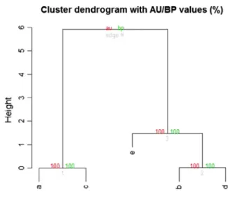
In addition, this procedure leaves researchers with data points nested within a tree structure based upon the merging of similar clusters. In the case of a survey measure, this produces a phylogenic-tree-like structure relating items within a survey to each other. A dendrogram, depicted in Fig. 2, shows the nested variable clusters found through hierarchical clustering; in this example, there are three clusters, two of which seem to be related. Variablesaandcform a unique cluster together, and variablesd

andbform a cluster that is closer to variablee than to thea/c

cluster. Variable e, contained within the b/d cluster, branches from a higher-up cluster containing all three related variables, showing the nesting structure that is present in hierarchical clustering.

Then the dissimilarity matrix used in this clustering method can be used to create a final heat map based upon final clusters extracted by the algorithm, with red denoting areas of varying degrees of similarity (darker represents more similarity) and with blue denoting areas of varying degrees of dissimilarity (darker rep-resents more dissimilarity;Fig. 3). In the sample heat map pre-sented inFig. 3, variables a and c are strongly similar to each other, as are variablesbandd; however, variablesaandcare dis-similar to variablee, whereas variablesbanddare similar to vari-ablee. These heat maps have allowed genomics researchers to identify genes that behave in a similar fashion with respect to a given outcome (e.g., disease, pathway activation, epigenetic change) through visual means, which may be much quicker and easier to interpret compared to sorting through pages of statistical output from hierarchical clustering on a large number of variables (Brown & Botstein, 1999; Wilkinson & Friendly, 2009).

In psychology, given these properties, the heat map provides a useful tool for analyzing complex constructs, where the researcher needs to cluster the interconnections between two variables and needs a visual tool easy to read, even with a big amount of data. This means that complex constructs can be analyzed in their artic-ulation without being oversimplified, as it occurs with traditional methods.

For less-statistically-inclined readers, an analogy from the field of music may be useful to understand what hierarchical clustering and its associated visual aids (i.e. the heat map and means plots) search for within a dataset. Sorting our data into these partitions is a bit like looking at classes of instruments (identity domains) and different movements (life contexts) across a collection of sym-phonies (study participants). The algorithm looks across the entire collection of symphonies to partition different types of instruments that are common overall or common within different types of movements. Some instruments are common to most symphonies and can be found across many movements within symphonies, which would tend to form a large cluster with many instruments and movements as a diverse, inclusive cluster (say, woodwinds and strings generally used in all movements of a symphony). Others are common across many symphonies within a particular type of movement (such as percussions, especially used in fast movements, as Allegros or Scherzos); this sort of cluster includes disparate symphonies tied together by the inclusion of the partic-ular movement. Others are unique to a small number of sym-phonies but prominently feature one or two main instruments (such as the celesta in The Nutcracker); these form a small, specific cluster indicative of a small subgroup within the population. Each of these clusters gives a snapshot of what instruments go into a

symphony and where one can usually find these instruments, as well as captures any of the more unique features of a small subset of the symphonies.

3. The present study

In the present study, we used both exploratory factor analysis (standard method for scale validation) and hierarchical clustering (our proposed method) with data collected using the ILLCQ, a fac-torially structured measure. We compared the utility of these methods in terms of the interpretability of the factors/clusters obtained through each method. We also performed heat mapping – a visual technique for inspecting and interpreting a cluster solu-tion – with a smaller subset of the sample to ascertain the validity of hierarchical clustering for scale validation in situations where the number of items approaches or exceeds the number of participants.

3.1. Method

3.1.1. Measure: the Identity Labels and Life Contexts Questionnaire (ILLCQ)

The survey used as an example for this article was constructed to answer two general questions about identity. Specifically, the survey is intended to (1) explore how many different ‘‘selves” young people acknowledge, in terms of sets of multidimensional interconnections between identity aspects and life contexts; and (2) determine how identity salience varies across life contexts. Because identity is a bridging construct that encompasses many different self-aspects, or identity domains, such as gender, sexual-ity, ethnicsexual-ity, career, family, and peer group (Picariello, Amodeo, & Schwartz, in preparation; Vignoles, Schwartz, & Luyckx, 2011), it is a priori unknown precisely how these different self-aspects are interconnected though contexts (Harter, 2012).

Put another way, followingErikson (1950), identity is expected to vary as a result of two primary factors – the specific identity domain being examined and the life context in which one finds oneself. The ILLCQ considers these two sources of variation together. Specifically, individuals are asked to rate the importance of each identity domain within a range of life contexts, where each domain-context pairing is assumed to be functionally independent from the others (i.e., no latent factors are posited as underlying the correlations between or among the pairings). For example, sexual orientation may be more salient within intimate relationships than in school or work, and religiosity may be more salient in a house of worship than in one’s peer group.

Our objective with the ILLCQ – and the objective within other factorially structured measures – is to classify responses (in this case domain-context pairings) within participants. Put differently, our objective is similar to the goal of heat mapping in genomics: to classify genes that behave in similar ways in the context of specific situations (e.g., diseases; Tabibiazar et al., 2005). Such within-participant clustering is not commonly performed in the social sciences, but it appears to match the structure and assumptions of the ILLCQ and other similarly structured measures.

Concretely, the ILLCQ consists of three distinct sections. The present study examines only the first section, which refers to Iden-tity Domain X Life Context pairings. This first section of the ILLCQ is represented as a 137 grid, where rows represent identity domains (gender, stage of life, socio-economic status, race, sexual orientation, school success, physical appearance, look, youth sub-cultures or tribes, political orientation, religious faith, music, and sport), and columns represent life contexts (family, school/job, neighborhood, peer group, spare time, religion, and dating). Respondents are invited to rate the extent to which, on a 1–5 scale,

each identity domain is important within each of their life contexts (seeFig. 1).

The ILLCQ was developed based on a qualitative assessment strategy introduced by Narváez, Meyer, Kertzner, Ouellette, and Gordon (2009), who conducted semi-structured interviews to study the intersections among sexual, ethnoracial, and gender identities espoused by minority group members, as well as how these identities are endorsed differently within different sociocultural contexts. Following typical methods for constructing and validating questionnaires (Dillman, Smyth, & Christian, 2009), we conducted focus group discussions with eight (4 females, 4 males) adolescents and young adults. Based on the responses from focus group participants, we adapted Narváez et al.’s qualitative measurement tool into a quantitative survey for self-administration.

3.1.2. Participants and procedures

The questionnaire was uploaded on the Qualtrics platform and posted onto the psychology participant pool using the SONA Sys-tems website at Florida International University (FIU). Participants received two hours of credit toward a research requirement (where a total of five research hours is required to pass the introductory psychology course). The ILLCQ was presented as part of an online

battery of measures (the ILLCQ was the first measure

administered).

The final sample included 406 participants, of which 80.8% self-identified as female, 19% as male, and 1 person (0.2%) as ‘‘other”. The average age of participants was 21.11 years (SD = 2.38). In terms of family education, 5.4% of fathers and the 3.5% of mothers had a doctoral degree; 12.2% of fathers and 10.3% of mothers had a master’s degree; 23.6% of fathers and 32.9% of mothers had a bach-elor’s degree; 42.3% of fathers and 41.5% of mothers had completed high school; 12% of fathers and 10.3% of mothers had attended some high school; and 3.8% of fathers and 1.5% of mothers had less than a 9th grade education. With reference to parents’ employ-ment, 6.9% of fathers and 9.8% of mothers were unemployed; 41.9% of fathers and 53% of mothers were employees; 24.3% of fathers and 15.7% of mothers were self-employed; the 6.1% of fathers and 3% of mothers were employed in manual labor; 14.8% of fathers and 4.8% of mothers were employees; 12.1% of mothers (but no fathers) were homemakers; and 5.9% of fathers and 1.5% of mothers were retired.

4. Exploratory factor analysis

First, we conducted Exploratory Factor Analyses (EFA) using an oblique rotation (i.e., Promax with Kaiser Normalization) in SPSS. For the EFA, the number of factors to retain was determined through consideration of (a) results of parallel analysis (Horn, 1965; Longman, Cota, Holden, & Fekken, 1989); (b) simple struc-ture (Thurstone, 1947); and (c) factor interpretability. Parallel analysis is a procedure that statistically determines the break in the scree plot (Horn, 1965; Longman et al., 1989); it produces more accurate factor extractions than the commonly used Kaiser’s (1960)eigenvalue > 1.0 rule (Zwick & Velicer, 1986). The parallel analyses were conducted in SPSS with syntax created by

O’Connor (2000) using both the mean eigenvalues and the 95th percentile eigenvalues (cf.Longman et al., 1989). In interpreting factors, a cutoff of0.30 was used to determine salient loadings.

4.1. EFA results

EFA indicated that a nine-factor solution was most viable (59.62% of variance explained). Rotated factor loadings are shown inTable 1. The model indicated 10 hyperplane items, or items that do not have salient loadings (>0.3) on any factors in the model and 4 complex items, or items with salient loadings on multiple factors (cross-loading). The nine-factors include two distinct identity-focused factors, Political Orientation (Factor 6) and Tribal Identity (Factor 7) in which all identity-context pairings for these identities loaded on a single factor. Religious Faith (Factor 1), in contrast, included all religious identity items across all contexts (other than religious places) along with all other identity items rated within religious contexts. Factor 9 included gender, age, sexual orienta-tion, beauty, look, and tribe domains within the dating context. The remaining factors included combinations across different

iden-tity domains and contexts: the socio-economic and racial/ethnic identities loaded onto a single factor across all contexts except for religious place (Factor 2), where this factor also included sexual orientation domain items within the school, neighborhood, and free time contexts. The Beauty and Look/Style domains (Factor 3) loaded together across contexts, except for the religious place con-text (for both beauty and look/style) and the dating concon-text (for beauty only). Factor 4 was a cross-identity/cross-context factor wherein Music domain in the free time, religious and dating con-texts loaded with the Sports domain in the family, school, neigh-borhood, and group contexts. The remaining Sports domain loaded onto Factor 8 on the free time, religious, and dating con-texts. Finally, the Gender and Age (Life Phase) domains loaded together across the family, school, group, and free time contexts (Factor 5).

5. Cluster analysis, hierarchical clustering, and heat mapping The cluster solution emerging from the hierarchical cluster analysis and depicted in the heat map may provide an answer to the first question that we posed regarding what ‘‘selves” might emerge from analysis of aspects-contexts pairings. In the hierarchi-cal cluster analysis and heat map, significant clusters represent the ‘‘selves” that respondents acknowledge, including specific domain-context pairings, and that may form the structure of identity as a bridging construct. This is an important answer both theoretically (for identity theory and research) and statistically (for the use of within-person hierarchical clustering and heat mapping in social-science research).

With respect to the second question – how mean levels of iden-tity salience vary within and across aspects and contexts – a simple line graph, illustrating the ways in which the self-reported impor-tance of each identity aspect varies across social contexts, can be

used to examine the interaction between self-aspects and the social contexts in which they may be expressed. This plot summa-rizes the pattern of means across identity domains, life contexts, and their interaction, whereas the heat map summarizes the pat-tern of similarities across identity domains, life contexts, and their interaction. In this case, heat maps are useful to illustrate which identity domains participants assign similar salience within a given life context. Both heat maps and means plots can be used

to graphically represent the inner workings of the hierarchical clustering.

To demonstrate the effectiveness of hierarchical cluster and heat map methodology with complex survey designs and small sample sizes where Nis approximately equal to the number of items, a random sample of 130 participants was drawn from the full sample. To examine how many distinct clusters of identity domain-life context pairings exist, we used both a visual heat

Table 1 EFA results. 1 2 3 4 5 6 7 8 9 Age_religion 0.792 0.010 0.055 0.158 0.225 0.103 0.101 0.025 0.091 Gender_religion 0.769 0.048 0.022 0.076 0.213 0.126 0.054 0.013 0.056 Religious_group 0.681 0.144 0.157 0.049 0.186 0.047 0.121 0.119 0.320 Sexual_Orientation religion 0.675 0.131 0.119 0.115 0.000 0.035 0.034 0.036 0.251 School_Success_religion 0.667 0.186 0.235 0.004 0.229 0.122 0.099 0.073 0.069 Religious_family 0.652 0.067 0.108 0.022 0.047 0.223 0.165 0.056 0.067 Look_religion 0.629 0.129 0.341 0.007 0.047 0.125 0.054 0.119 0.050 Religious_freetime 0.627 0.048 0.125 0.099 0.004 0.222 0.158 0.130 0.281 Beauty_religion 0.585 0.162 0.387 0.069 0.057 0.038 0.037 0.064 0.057 Religious_neighborhood 0.579 0.056 0.009 0.090 0.145 0.269 0.176 0.035 0.051 Religious_school 0.566 0.008 0.018 0.050 0.149 0.305 0.246 0.049 0.046 Status_religion 0.557 0.131 0.031 0.087 0.021 0.015 0.005 0.012 0.193 Race_religion 0.527 0.311 0.110 0.050 0.018 0.039 0.072 0.115 0.002 Political_dating 0.503 0.101 0.154 0.180 0.201 0.086 0.144 0.294 0.116 Music_neighborhood 0.489 0.058 0.087 0.246 0.031 0.072 0.036 0.020 0.137 Tribes_religion 0.470 0.042 0.096 0.104 0.008 0.033 0.517 0.040 0.010 Sport_neighborhood 0.416 0.015 0.018 0.645 0.147 0.088 0.042 0.141 0.163 Gender_neighborhood 0.404 0.115 0.246 0.105 0.264 0.113 0.101 0.195 0.058 Race_school 0.003 0.718 0.107 0.010 0.142 0.028 0.003 0.254 0.083 Race_group 0.025 0.676 0.032 0.036 0.055 0.091 0.026 0.030 0.053 Race_neighborhood 0.269 0.641 0.068 0.140 0.006 0.060 0.103 0.037 0.082 Race_freetime 0.050 0.584 0.097 0.006 0.024 0.082 0.003 0.001 0.183 Race_dating 0.097 0.575 0.010 0.033 0.078 0.077 0.052 0.038 0.316 St_dating 0.092 0.556 0.049 0.059 0.023 0.117 0.016 0.071 0.230 Status_school 0.148 0.552 0.174 0.053 0.386 0.064 0.074 0.112 0.027 Status_freetime 0.143 0.529 0.000 0.005 0.174 0.100 0.010 0.079 0.006 Status_group 0.089 0.527 0.122 0.038 0.184 0.205 0.079 0.113 0.002 Status_neighborhood 0.153 0.520 0.043 0.132 0.133 0.082 0.112 0.109 0.082 Sexual_Orientation school 0.104 0.470 0.122 0.082 0.051 0.057 0.007 0.039 0.111 Race_family 0.010 0.463 0.155 0.063 0.226 0.076 0.025 0.255 0.002 Status_family 0.157 0.437 0.048 0.062 0.415 0.026 0.065 0.006 0.088 Sexual_Orientation neighborhood 0.343 0.412 0.224 0.034 0.126 0.037 0.032 0.150 0.012 Sexual_Orientation freetime 0.147 0.410 0.168 0.066 0.114 0.166 0.118 0.164 0.037 Beauty_neighborhood 0.261 0.100 0.725 0.005 0.039 0.020 0.049 0.082 0.039 Look_neighborhood 0.284 0.095 0.713 0.060 0.016 0.005 0.039 0.050 0.006 Beauty_group 0.099 0.091 0.712 0.015 0.194 0.170 0.066 0.009 0.156 Look_group 0.117 0.053 0.670 0.047 0.199 0.129 0.090 0.004 0.249 Beauty_freetime 0.004 0.036 0.653 0.021 0.099 0.095 0.044 0.045 0.029 School_Success_group 0.000 0.276 0.623 0.052 0.159 0.023 0.142 0.132 0.146 Look_family 0.059 0.095 0.606 0.060 0.177 0.047 0.026 0.205 0.132 Beauty_school 0.001 0.083 0.578 0.158 0.052 0.005 0.000 0.259 0.016 Look_freetime 0.037 0.059 0.569 0.019 0.200 0.056 0.012 0.037 0.019 Look_school 0.000 0.089 0.554 0.040 0.226 0.019 0.075 0.193 0.004 School_Success_neighborhood 0.284 0.276 0.538 0.028 0.227 0.116 0.058 0.072 0.085 Beauty_family 0.092 0.016 0.479 0.098 0.136 0.042 0.039 0.246 0.095 Look_dating 0.024 0.015 0.476 0.103 0.008 0.056 0.070 0.084 0.534 School_Success_dating 0.071 0.216 0.471 0.083 0.295 0.025 0.029 0.154 0.293 Sport_family 0.024 0.054 0.026 0.928 0.082 0.006 0.098 0.154 0.156 Music_religion 0.037 0.045 0.023 0.846 0.099 0.015 0.106 0.021 0.113 Music_freetime 0.013 0.009 0.072 0.842 0.093 0.019 0.023 0.026 0.162 Sport_group 0.093 0.019 0.047 0.826 0.151 0.097 0.083 0.079 0.188 Sport_school 0.013 0.052 0.115 0.815 0.003 0.007 0.065 0.061 0.119 Music_dating 0.216 0.058 0.054 0.640 0.178 0.029 0.162 0.134 0.070 Gender_group 0.068 0.005 0.159 0.118 0.633 0.076 0.034 0.188 0.151 Age_family 0.131 0.042 0.101 0.043 0.591 0.146 0.077 0.179 0.076 Age_school 0.077 0.137 0.078 0.109 0.584 0.200 0.167 0.135 0.105 Age_freetime 0.046 0.127 0.012 0.062 0.579 0.070 0.118 0.245 0.069 Age_group 0.113 0.007 0.155 0.154 0.574 0.069 0.040 0.224 0.250 Gender_family 0.192 0.048 0.089 0.137 0.553 0.007 0.009 0.153 0.171 Gender_freetime 0.164 0.065 0.117 0.047 0.536 0.027 0.070 0.177 0.084 Gender_school 0.134 0.189 0.124 0.087 0.496 0.113 0.066 0.076 0.193 Political_neighborhood 0.125 0.080 0.056 0.065 0.068 0.965 0.058 0.086 0.002 Political_family 0.103 0.038 0.015 0.004 0.035 0.773 0.130 0.114 0.077 Political_group 0.077 0.058 0.121 0.009 0.062 0.760 0.146 0.087 0.159 Political_religion 0.025 0.117 0.013 0.014 0.163 0.731 0.076 0.055 0.236 Political_school 0.127 0.046 0.096 0.129 0.142 0.729 0.144 0.005 0.012 Political_freetime 0.323 0.001 0.072 0.032 0.089 0.562 0.088 0.037 0.025 Tribes_dating 0.092 0.015 0.040 0.172 0.007 0.007 0.717 0.452 0.165 Tribes_freetime 0.121 0.020 0.029 0.069 0.172 0.133 0.688 0.058 0.096 Tribes_neighborhood 0.146 0.040 0.066 0.030 0.038 0.130 0.671 0.062 0.022 Tribes_school 0.100 0.003 0.009 0.159 0.106 0.050 0.666 0.008 0.237 Tribes_group 0.134 0.024 0.045 0.159 0.181 0.139 0.645 0.251 0.034 Tribes_family 0.052 0.028 0.052 0.090 0.163 0.131 0.616 0.099 0.194 Beauty_dating 0.079 0.017 0.308 0.047 0.064 0.004 0.110 0.640 0.083

map of the data and a hierarchical clustering algorithm capable of testing significant boundaries within the dendrogram. To create the heat map, the R packagepheatmap was used, which allows users to create heat map colors, choose the type of hierarchical clustering method, and control the graphical parameters. This allows users to customize their heat map according to the needs of the study. This heat map was created using Ward’s algorithm, with squared Euclidean distances and the pairwise complete option for missing data (in which all observations with valid values for both variables in a given pair are used), with the traditional red-orange color used to depict smaller squared Euclidean distances and blue used to depict larger squared Euclidean distances. Although there are numerous hierarchical clustering methods, across a wide-range of simulation studies it has often been found that Ward’s method provides perhaps the most stable and inter-pretable results. Ward’s method creates clusters such that, at each merger, the merger minimizes the increase in the sum-of-squares error – which is essentially the numerator for the variance. Thus, Ward’s clustering attempts to create a set of clusters with mini-mum variance, mapping onto the notion that clusters should be internally cohesive and externally isolated (Cormack, 1971).

Though heat maps can be used to depict correlation, this heat map uses a similarity-based measure. The intensity of color for an individual item with itself gives an indicator of main effects; the shade and intensity of an item with another item gives an indi-cator of possible interaction between the two items; and the over-all intensity and hue provide an indication of underlying structure of the measure across many items. This analytic procedure was repeated an additional four times to assess the stability of this method in identifying important subgroupings of survey items through cross-validation. Sampling was done without replacement within the full sample, using thesamplefunction in R.

To test for the significance of nested clusters (i.e., the extent to which a group of item responses are more similar to one another than to other item responses), the R package pvclust was used, employing the same hierarchical clustering algorithm parameters as those used to create the heat map. This algorithm can test for significance via bootstrap probability estimates and a newer varia-tion of bootstrapping called multi-scale bootstrap resampling, which provides approximately unbiased probability estimates for each clustering (Suzuki & Shimodaira, 2006). In addition, this pack-age provides graphical diagnostics for bootstrap estimates and a dendrogram (tree) showing nested clusters and boxes around each significant cluster for a given significance level, as well as output denoting variable names contained within each significant cluster,

which can be difficult to read on large heat maps and dendrograms. Thepvpickfunction was then applied to obtain information about variable inclusion within significant clusters. This allowed us to characterize significant relationships among our identity measures and to compare significant cluster trends to extant theories of identity.

To answer the question of whether or not the reported impor-tance of identity aspects varies across social contexts as well as the magnitude of such variations, we examined the significant clusters found by thepvpickfunction, as well as the plotted mean identity score for each of the 13 identity aspects across all seven contexts. If identity is constant over context, the mean plot should show a fairly flat line across the seven contexts; if it varies by con-text, at least one point on the graph will show a large spike or drop from the straight line. In addition, if identity is constant over con-text, identity questions will cluster based on aspects of identity (on gender, for example), rather than based on contexts. Hence, if iden-tity importance varies by aspect but not by context, a single cluster would be expected to include questions about a specific context (the school context, for example), notwithstanding the identity domain being considered (in our example, we expect to find like level of importance assigned to gender, age, religion, ethnicity, etc. in relation to the school context).

5.1. Cluster analytic results

To compare results across cross-validation samples, a nonpara-metric statistical test was developed using the Hausdorff nonpara-metric (Burago, Burago, & Ivanov, 2001; Geetha, Ishwarya, & Kamaraj, 2010). Hausdorff distance is a topological measure of relation between two objects within the same dimensional space; in essence, it represents the furthest possible distance from one object to another (Geetha et al., 2010). Several nonparametric tests between statistical objects other than datasets themselves have been developed in recent years, including Wasserstein distance for histograms and persistence diagrams (Bubenik, 2015) and Gromov-Hausdorff distance for shape matching (Chazal et al., 2009). Distance is measured between two objects of interest; then, a random distribution of distances is generated through either object permutations or random object generation to derive a prob-ability density function. From this distribution, it is possible to sta-tistically test the distance between objects to determine if they are different from each other. The Hausdorff method thus represents a generalization of traditional nonparametric methods to a richer set of statistical objects. Here, we test equivalence of dendrograms

Table 1(continued) 1 2 3 4 5 6 7 8 9 Age_dating 0.121 0.067 0.089 0.071 0.192 0.021 0.156 0.584 0.065 Sexual_Orientation dating 0.070 0.183 0.053 0.059 0.090 0.033 0.018 0.556 0.001 Gender_dating 0.135 0.073 0.072 0.019 0.251 0.023 0.107 0.521 0.154 Sport_religion 0.083 0.023 0.030 0.210 0.092 0.089 0.223 0.096 0.821 Sport_freetime 0.111 0.060 0.060 0.037 0.127 0.034 0.182 0.041 0.815 Sport_dating 0.349 0.075 0.169 0.286 0.215 0.062 0.153 0.094 0.690 School_Success_school 0.126 0.100 0.271 0.024 0.110 0.218 0.077 0.273 0.415 Sexual_Orientation family 0.171 0.287 0.040 0.078 0.096 0.082 0.059 0.099 0.210 Sexual_Orientation group 0.133 0.345 0.151 0.068 0.101 0.180 0.064 0.123 0.094 School_Success_family 0.142 0.167 0.285 0.044 0.025 0.179 0.135 0.172 0.399 School_Success_freetime 0.046 0.282 0.368 0.145 0.006 0.001 0.071 0.066 0.010 Age_neighborhood 0.352 0.133 0.247 0.219 0.166 0.108 0.263 0.065 0.184 Religious_religion 0.071 0.030 0.138 0.344 0.242 0.039 0.005 0.266 0.116 Religious_dating 0.026 0.158 0.199 0.341 0.180 0.009 0.030 0.234 0.045 Music_family 0.067 0.042 0.194 0.380 0.284 0.036 0.043 0.093 0.174 Music_school 0.001 0.058 0.175 0.292 0.302 0.086 0.057 0.023 0.069 Music_group 0.062 0.039 0.248 0.305 0.178 0.084 0.077 0.235 0.105 Italics refer to significant values.

based on random samples of this study’s survey participants to determine the stability of our proposed method. A p-value > 0.05 suggests that the dendrograms are topologically close enough to conclude that results are similar across samples.

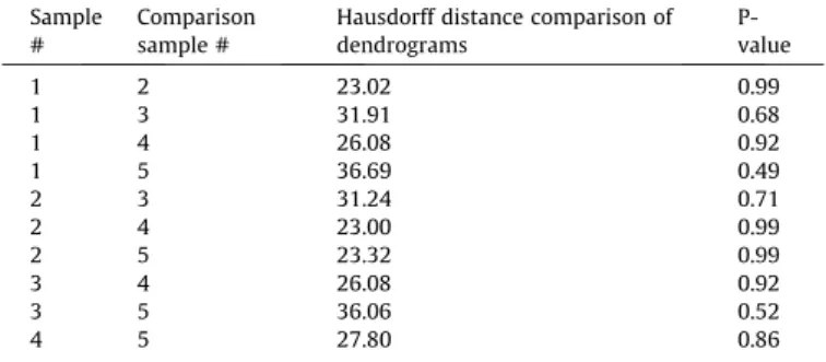
Five samples of 130 participants were randomly drawn, with replacement, from the full sample. The results for each randomly drawn sample were compared against each other sample. Haus-dorff distances between sample dendrograms were calculated and compared against a generated distribution of random tree pairs to obtain a p-value. A Bonferroni correction was applied to account for multiple testing.Table 2provides the results, which suggest that the dendrogram structures are consistent across ran-domly selected samples.

These nonsignificant differences are reflected both in the heat maps and in the hierarchical clustering tests, which indicated quite similar patterns and suggested that this method is fairly stable across samples drawn from the same population. Because results were not significantly different across samples, the first sample analyzed was chosen for in-depth review of results, and accompa-nying graphics are based on this sample for brevity. The heat map (Fig. 4) shows several blocks of strong similarities. Some of these (such as tribe) seem to represent islands of similarity, whereas other aspects are more widely similar to one another (e.g., beauty

and look) or to several other aspects (such as race/gender/age and look/beauty/gender/status). In each cluster, whether individually or clustering with other variables, the greatest similarities appear to be within identity domains across contexts (e.g., tribe in the peer context with tribe in other contexts). Interestingly, context does not seem to matter much in many of these preferred clusters, though some exceptions do stand out, as in the contexts of neigh-borhood and religion.

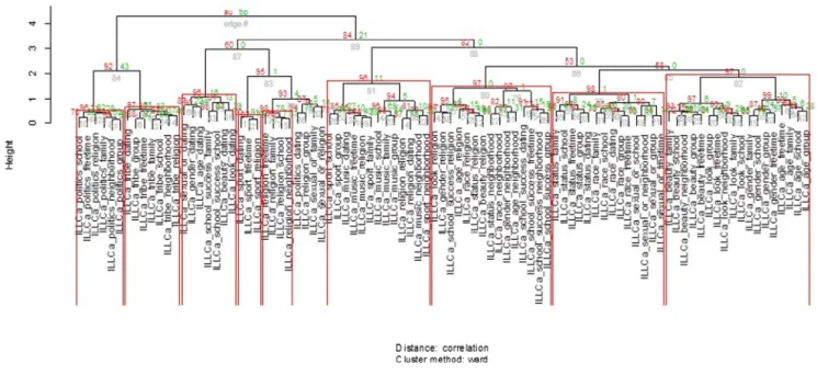
The hierarchical clustering algorithm extracted nine clusters, significant at the 0.05 level, that correspond well with the heat map’s ascertainment of important variables. As illustrated in

Fig. 4, the first includes sport in the contexts of free time, religion, and dating. The second includes religion across family, school, neighborhood, and free time. The third includes politics across six different contexts. The fourth includes all seven contexts of tribe, showing a strong preference for identity domain over con-text. The fifth consists of age, gender, look, sexual orientation, and beauty within the context of dating, as well as school success in the contexts of school and family. The sixth includes several demographic characteristics (status, race, and sexual identity) across many contexts. The seventh consists of school success across many contexts and several identities within the contexts of neighborhood and religion. The eighth includes religion, sport, and music across many contexts as a sort of ‘‘leisure activity clus-ter”. The final is a mixture of demographic (age, gender) and phys-ical (beauty, look) characteristics across social group settings. These relationships are summarized using a dendrogram with sig-nificant nested clusters circled in red (Figs. 4 and 5), as well as a table-based list (Table 3, which also includes a contrast to the EFA Factor solution). Significance aside, the dendrogram also sug-gests that identity domain is more important than life context in the creation of clusters in most cases; however, the fifth and sev-enth clusters seemed to favor context over identity type, suggest-ing that religious contexts may create more similarity across identity aspects than other types of contexts.

To test dendrogram similarity and to verify that clusters exist in a non-random pattern, we used the cophenetic correlation. The

Table 2

Test of hierarchical clustering differences among samples. Sample

#

Comparison sample #

Hausdorff distance comparison of dendrograms P-value 1 2 23.02 0.99 1 3 31.91 0.68 1 4 26.08 0.92 1 5 36.69 0.49 2 3 31.24 0.71 2 4 23.00 0.99 2 5 23.32 0.99 3 4 26.08 0.92 3 5 36.06 0.52 4 5 27.80 0.86

cophenetic correlation is used to compare the heights between all pairs of dendrograms, and, for all five samples, these were moder-ate. To test difference from zero, a random permutation program was developed, such that, for each pair of ‘‘dendrograms”, one was held constant while the other was randomly permuted 1000 times to simulate a null relationship. These gave 95% confidence

bounds for each pair; none of the observed values fell within this range, suggesting that consistent structure exists across samples.

As expected from the cluster results, the means plot (Fig. 6) also suggests that most identity domains are fairly stable over many different contexts, supporting the hierarchical clustering results and suggesting that the graphical methods are convergent.

Fig. 5.Cluster dendrogram.

Table 3

Significant clusters and factors summary Closest factor analogue Cluster

number

Domain-context intersections Factor number

Description of difference from cluster solution

Cluster 1 3-items

Sport-Freetime, Sport-Religion, Sport-Dating Factor 8 3-items

Identical to Cluster 1 Cluster 2

4-items

Family, School, Neighborhood, Religion-Freetime

Factor 1 18-items

Factor also has Religion-Group and the religious context of Gender, Religion, Age, Status, Race, Sexual, Beauty, Look and the Neighborhood context of Gender, Music and Sport as well as Politics-Dating

Cluster 3 6-items

Family, Neighborhood, School, Politics-Group, Politics-Freetime, Politics-Religion

Factor 6 6-items

Identical to Cluster 3 Cluster 4

7-items

Tribe-Family, Tribe-School, Tribe-Dating, Tribe-Neighborhood, Tribe-Group, Tribe-Freetime, Tribe-Religion

Factor 7 7-items

Identical to Cluster 4 Cluster 5

7-items

Gender-Dating, Age-Dating, School School, School Success-Family, Beauty-Dating, Look-Dating, Sexual-Dating

Factor 9 6-items

5 items overlap, does not contain School Success-School, School Success-Family and does include a cross-loading of Tribe-dating Cluster 6

14-items

Status-Family, Status-School, Status-Group, Status-Freetime, Status-Dating, Family, School, Group, Race-Freetime, Race-Dating, School, Group, Sexual-Neighborhood, Sexual-Freetime

Factor 2 15-items

13 items overlap. The Sexual-Group items of Cluster 6 is not in Factor 2. Factor 2 includes Status-Neighborhood and Race-Neighborhood which Cluster 6 does not

Cluster 7 15-items

Gender-Neighborhood, Neighborhood, Gender-Religion, Age-Religion, Status-Neighborhood, Status-Age-Religion,

Race-Neighborhood, Race-Religion, School Success-Race-Neighborhood, School Group, School Freetime, School Success-Religion, School-Success Dating, Beauty-Success-Religion, Look-Religion

Factor 3 14-items

3 items overlap (School Neighborhood, School Success-Group, School-Success Dating). Factor 3 does not include: Gender-Neighborhood, Age-Gender-Neighborhood, Gender-Religion, Age-Religion, Status-Neighborhood, Status-Religion, Neighborhood, Race-Religion, School Success-Freetime, School Success-Religion. Factor 3 does include: Beauty and Look (style) identities in the family, school, neighborhood, group and freetime contexts

Cluster 8 11-items

Music-Family, Music-School, Music-Neighborhood, Music-Group, Music-Freetime, Music-Religion, Music-Dating, Sport-Family, Sport-School, Sport-Neighborhood, Sport-Group

Factor 4 7-items

The 7 items of Factor 4 are all in Cluster 8. The following items of Cluster 8 are not included in Factor 4: Music-Family, Music-School, Music-Neighborhood, Music-Group

Cluster 9 16-items

Gender-Family, Gender-School, Gender-Group, Gender-Freetime, Age-Family, Age-School, Age-Group, Age-Freetime, Beauty-Family, Beauty-School, Beauty-Freetime, Family, School, Look-Neighborhood, Look-Group, Look-Freetime

Factor 5 9-items

Includes all Gender and Age identity items as cluster 9 but none of the Beauty or Look items, also has a cross-loading on Status-Family

However, some contexts seem to have a stronger effect over iden-tity domains than others do. There does seem to be a context effect for all domains of identity within a religious context, and, in partic-ular, it appears that this pattern interacts with sexual and sport identity. In addition, there seems to be a context-identity interac-tion effect for music within the school, neighborhood, free time, and dating contexts. In addition, sport and religious identity seem to show the opposite trend from that for the other identities within the dating context, suggesting a context-identity effect for the sport and religious identity domains. Given that sport and religion were also split between clusters, this visual pattern is consistent with the clustering results.

These findings suggest that a means plot similar to this one may help be a useful visual tool to better understand the complex and composite nature of identity and that a plot similar to this is con-vergent to the results found by the hierarchical clustering analyses. In a way, this is akin to a graphical/qualitative ANOVA when too few participants exist to test interaction effects and group differ-ences through an ANOVA. This sequence of analyses provides users of hierarchical clustering a more familiar graphical display of main effects and interactions within their dataset.

6. Discussion

These results suggest that hierarchical clustering and various related graphical tools – the heat map, the dendrogram, and the means plots – provide a viable alternative to traditional methods examining the structure and mean levels of factorially structured surveys intended to analyze bridging constructs such as identity. These results appear to be stable over multiple samples, analyti-cally tractable when sample size is small relative to survey size, and statistically testable (providing a p-value for groupings within a statistical method that is not wholly parametric). These methods provide social science researchers with valuable tools with which to analyze and assess complex self-report measures, and opens the door to survey-designers with nontraditional designs, such as the factorially-structured ILLCQ.

Comparing the EFA and hierarchical clustering approaches sug-gested considerable overlap in the clusters/factors identified. How-ever, there were also distinct differences in several areas involving the interaction between identity domains and life contexts. For example, Cluster 6 appeared to represent clustering of the

Neigh-borhood and Religion contexts across the Gender, Age, Race and School Success domains (this grouping did not emerge from the factor solution). Similarly, Cluster 9 was characterized by a conflu-ence among the Gender, Age, Beauty and Look (style) domains across the Family, School, Group and Freetime contexts. Factor 4, the closest match for this cluster within the EFA solution, only par-tially suggested such a confluence – specifically, in the EFA solu-tion, the Beauty and Look domains were not linked with the Gender and Age domains within the Family, School, Group, and Freetime contexts. It might be reasonable to argue that gender, age, and physical appearance are part of the ‘‘public identity” that one uses to present oneself to others (Meca et al., 2015). The clus-ter solution was able to produce a grouping reflecting this type of public identity within specific interpersonal contexts, but the fac-tor solution was not.

It is important to note that, for the EFA solution, there were only about 4.5 observations per item included in the analysis, far below the number recommended for a stable EFA solution. This limited sample size also precludes splitting the sample in half to conduct EFA on the first half and confirm the solution on the second half with CFA. In contrast, for the hierarchical clustering solution, we were able to include cross-validation with a statistical evaluation of both the replication stability and the fit of the clustering solution.

This study is the first of its kind to implement hierarchical clus-tering as an analytical tool for measurement validation, as first pro-posed by Revelle in 1979, and, as such, this study provides valuable insight into the application of this method to psychometric analy-ses, as well as a starting point for the development of this sort of method for the analysis of factorially-designed surveys.

Although the purpose of the present study was primarily methodological, it may be possible to state some innovative impli-cations of the results for identity theory as well. First, the heat map, which indicates more dissimilarity than similarity across identity domains and life contexts, suggests that identity is more likely a bridging construct than a higher-order construct. Such a conclu-sion is bolstered by inspection of the means plot, which suggests different patterns of differences across contexts for most of the identity domains. The fact that the EFA model diverged from the cluster solution in important ways (e.g., overlooking subtleties involving convergence between or among identity domains within specific life contexts) provides additional support for our conclu-sion. For example, various aspects of public identity (e.g., physical

appearance, gender, socioeconomic status) would be expected to cluster together – yet this occurred only within the hierarchical cluster analyses, and not in the EFA results.

Erikson (1950, 1968)spoke of identity as a dynamic interplay between the person and her/his social and cultural context, such that specific contexts elicit certain identity-related responses from young people. Empirical research has largely supported this propo-sition (see Bosma & Kunnen, 2008). Many identity domains are connected to groups that exist and are brought together thanks to those specific aspects – for example, sexual orientations are con-nected to groups (i.e., groups of heterosexual, bisexual, or homo-sexual people), genders are connected to groups (groups of women, of men, of transsexual people, etc.), ethnicities are con-nected to groups (Caucasian, Black, Asian groups, etc.), religions are connected to groups (Catholic, Muslim, Buddhist, etc.), and so on. Social-psychological research indicates that different social contexts bring out specific group identifications, and that individ-uals respond differently depending on the specific group identity aspect that has been elicited (Ellemers et al., 2002; Scandurra, Braucci, Bochicchio, Valerio, & Amodeo, 2017; Scandurra, Picariello, Valerio, & Amodeo, 2017). For example, Settles, Jellison, and Pratt-Hyatt (2009)found that, among female scien-tists, increases in scientist identity, but not female identity, were predictive of self-esteem over time. The ILLCQ allows us not only to consider the activation of different identity domains, but also to do so across a range of life contexts. The ILLCQ, and the analyses that can be used to analyze data generated by this measure, may therefore come closer to analyzing Erikson’s person-context inter-play than any other measure that has been introduced thus far.

The methodological advances that the present study offers may therefore allow for theory testing and measurement validation beyond what is possible using traditional factor-analytic or item-response techniques. Rather than limiting ourselves to designing measures whose data can be analyzed using available statistical methods, it may be preferable to create measures that provide the means to test theory most precisely and then develop, adapt, or translate statistical techniques to analyze data generated from the measure. As a result, another potential contribution of our study may be to broaden the range of statistical techniques avail-able for measurement validation.

7. Limitations

The present results should be considered in light of several important limitations. First, the present sample consists largely of U.S. college students, and as such, we do not know whether sim-ilar results would have emerged with other age groups or with young adults not attending college. Second, our sample was largely female, and it is important to replicate the present results with a more gender-balanced sample. Third, the study was cross-sectional, while assessment of change over time would have pro-vided information as to the extent to which the measurement structure of the ILLCQ (and assumedly the structure of identity) is consistent over time.

There are also limitations inherent in the use of cluster analytic methods. The primary limitation of hierarchical clustering, and cluster analysis in general, is that it is an exploratory technique. As a result, there is always a possibility that the method over-capitalizes on chance. Within the analyses reported here, this potential capitalization on chance is somewhat mitigated by both (a) the bootstrap procedure utilized in pvclust and (b) dividing the dataset into multiple sub-samples and repeating the analysis on each sub-sample. However, as with all statistical procedures, replicability can best be shown by fitting the proposed final model to other, independent data sets. Beyond these concerns, caution

must be taken when utilizing hierarchical clustering as it imposes a hierarchical constraint on the final cluster solution. In the current study, we viewed that the hierarchical constraint as appropriate because it reflects the topological nature of ‘‘bridging” construct that was hypothesized.

Despite these and other potential limitations, the present study has provided important information on a new statistical method for validating measures of bridging constructs. Our study may help to begin to realize the potential of hierarchical cluster analysis and heat mapping in scale validation, as well as to introduce new ways of measuring constructs that are not predicated on a traditional factorial structure. We hope that our study helps to open a new line of work on bridging constructs, factorially based measures, and their validation.

References

Aggarwal, C. C. (2013). An introduction to cluster analysis. InData clustering: Algorithms and applications(pp. 1–28).

Baraniuk, R. G., & Wakin, M. B. (2009). Random projections of smooth manifolds.

Foundations of Computational Mathematics, 9(1), 51–77.

Bosma, H. A., & Kunnen, E. S. (2008). Identity-in-context is not yet identity development-in-context.Journal of Adolescence, 31(2), 281–289.http://dx.doi. org/10.1016/j.adolescence.2008.03.001.

Brown, P. O., & Botstein, D. (1999). Exploring the new world of the genome with DNA microarrays.Nature Genetics, 21, 33–37.

Brown, T. A. (2006).Confirmatory factor analysis for applied research. New York, N.J.: Guilford Press.

Burago, D., Burago, Y., & Ivanov, S. (2001).A course in metric geometry(Vol. 33 (pp. 371–374). Providence: American Mathematical Society.

Chen, F. F., Hayes, A., Carver, C. S., Laurenceau, J. P., & Zhang, Z. (2012). Modeling general and specific variance in multifaceted constructs: A comparison of the bifactor model to other approaches.Journal of Personality, 80, 219–251.http:// dx.doi.org/10.1111/j.1467-6494.2011.00739.x.

Cormack, R. M. (1971). A review of classification.Journal of the Royal Statistical Society, 134, 321–367.

Diamantopoulos, A., & Siguaw, J. A. (2006). Formative versus reflective indicators in organizational measure development: A comparison and empirical illustration.

British Journal of Management, 17(4), 263–282. http://dx.doi.org/10.1111/ j.1467-8551.2006.00500.x.

Dillman, D. A., Smyth, J. D., & Christian, L. M. (2009).Internet, mail, and mixed-mode surveys: The tailored design method(3rd ed.). Hoboken, NJ: Wiley.

Dimitrov, D. M., & Atanasov, D. V. (2011). Conjunctive and disjunctive extensions of the least squares distance model of cognitive diagnosis. Educational and Psychological Measurement.http://dx.doi.org/10.1177/0013164411402324. Ellemers, N., Spears, R., & Doosje, B. (2002). Self and social identity.Annual Review of

Psychology, 53, 161–186. http://dx.doi.org/10.1146/annurev. psych.53.100901.135228.

Erikson, E. H. (1950). Growth and crises of the ‘‘healthy personality”. In M. J. E. Senn (Ed.),Symposium on the healthy personality(pp. 91–146). Oxford, England: Josiah Macy, Jr. Foundation.

Erikson, E. H. (1968).Identity: Youth and crisis. New York: Norton.

Fabrigar, L. R., Wegener, D. T., MacCallum, R. C., & Strahan, E. J. (1999). Evaluating the use of exploratory factor analysis in psychological research.Psychological Methods, 4(3), 272.http://dx.doi.org/10.1037/1082-989X.4.3.272.

Floyd, S. W., Cornelissen, J. P., Wright, M., & Delios, A. (2011). Processes and practices of strategizing and organizing: Review, development, and the role of bridging and umbrella constructs. Journal of Management Studies, 48(5), 933–952.http://dx.doi.org/10.1111/j.1467-6486.2010.01000.x.

Ford, J. K., MacCallum, R. C., & Tait, M. (1986). The application of exploratory factor analysis in applied psychology: A critical review and analysis. Personnel Psychology, 39(2), 291–314. http://dx.doi.org/10.1111/j.1744-6570.1986. tb00583.x.

Fraley, C. (1998). Algorithms for model-based Gaussian hierarchical clustering.

SIAM Journal on Scientific Computing, 20(1), 270–281.http://dx.doi.org/10.1137/ S1064827596311451.

Geetha, S., Ishwarya, N., & Kamaraj, N. (2010). Evolving decision tree rule based system for audio stego anomalies detection based on Hausdorff distance statistics. Information Sciences, 180(13), 2540–2559. doi:0.1016/j. ins.2010.02.024.

Golub, G. H., & Reinsch, C. (1970). Singular value decomposition and least square solutions.Numerische Mathematik, 14(5), 403–420.

Güler, C., Thyne, G. D., McCray, J. E., & Turner, K. A. (2002). Evaluation of graphical and multivariate statistical methods for classification of water chemistry data.

Hydrogeology Journal, 10(4), 455–474.

Guo, D. (2003). Coordinating computational and visual approaches for interactive feature selection and multivariate clustering. Information Visualization, 2(4), 232–246.

Harter, S. (2012). Emerging self-processes during childhood and adolescence. In M. R. Leary & J. P. Tangney (Eds.), Handbook of self and identity (2nd ed., pp. 680–715). New York: Guilford Press.