Path-Loss Prediction for UHF/VHF Signal Propagation in Edo State: Neural Network Approach

(1)

ISSN: 2528-2417

DOI: 10.11591/APTIKOM.J.CSIT.17  77

Path-Loss Prediction for UHF/VHF Signal Propagation in

Edo State: Neural Network Approach

Ogbeide K. O.*, Eko Mwenrenren E. J.

Electrical/Electronic Engineering Department, University of Benin, P.M.B. 1154, Nigeria *Corresponding author, email: [email protected]

Abstract

The aim of this paper is to present and evaluate artificial neural network model used for path loss prediction of signal propagation in the VHF/UHF spectrum in Edo state.Measurement data obtained from three television broadcasting stations in Edo state, operating at 189.25MHz, 479.25MHz, and 743.25MHz, is used to train and evaluate the artificial neural network. A two layer neural network with one hidden and one output layer is evaluated regarding prediction accuracy and generalization properties. The path loss prediction results obtained by using the artificial neural network model are evaluated against the Hata and Walfisch-Ikegami empirical path loss models .Result analysis shows that the artificial neural network performs well as regards to prediction accuracy and generalization ability. The ANN performed better across all performance measures in comparison to the Hata and Walfisch-Ikegami and Line of Sight models in estimating path loss in vhf/uhf spectrum in Edo state.

Keywords: ANN, Hata-model, Pathloss, back-propagation, neurons

1. Introduction

Path loss is a major component in the analysis and design of the link budget of a telecommunication system. An accurate prediction of the path loss is usually necessary in building base stations or transmitting stations with optimized characteristics, such as position, height, transmitted power, and antenna pattern. Traditionally, path loss prediction models have been based on empirical and/or deterministic methods. Empirical models, such as Walfisch-Ikegami, Okumura, and Okumura– Hata models are computationally efficient [1], but may not be very accurate since they do not explicitly account for specific propagation phenomena. On the other hand, deterministic models, such as those based on the geometrical theory of diffraction integral equation and parabolic equation [2] can be very accurate but significantly more expensive in computational effort [3]. Therefore, artificial neural networks (ANNs) have been proposed in order to obtain prediction models that are more accurate than standard empirical models whilst being easier to compute than deterministic models. In recent years, ANNs have been shown to successfully perform path loss predictions in rural [4], suburban [5], urban [6] and indoor [7] environments. An Artificial Neural Network (ANN) prediction model can be trained to perform well in environments similar to where the training data is collected. Therefore, to obtain an ANN model that is accurate and generalizes well, measurement data from many different environments should be used in the training process. A multilayer feed-forward network with back-propagation can generally be used to solve function fitting or function approximation problems. This approximation ability can be applied to path loss prediction. Empirical path loss models are based on measured and averaged losses along typical classes of radio links. The Free Space loss model only takes into consideration distance and frequency. Hence, this model is very limited in its ability to accurately predict path loss in most environments [8].

( ) ( ) (1)

The Hata model is an empirical formulation of the graphical path loss data provided by Okumura. Hata presented the urban propagation loss as a standard formula and supplied correction Equations for application to other situations. The model can be described by the following Equations and parameters:

(2)

Carrier Frequency: 150 MHz ≤ fc ≤ 1500 MHz

Base Station Height: 30m ≤ hb ≤ 200m

Mobile Station Height: 1m ≤ hm ≤ 10m

T-R distance: 1km ≤ d ≤ 20km

Lp={

( )

A=69.55 + 26.16 log10 (fc) – 13.82 log10 (hb) – a (hm)

B=44.9 – 6.55 log10 (hb) C=5.4 + 2[log10 (fc / 28)] 2 D=40.94 + 4.78 [log10 (fc)] 2 – 18.33 log10 (fc) ( ) { [ ( ) ] ( ) [ ( )] [ ( )]

Hata’s model is based on measurements in Tokyo, Japan.

The WIM has been shown to be a good fit to measured propagation data for frequencies in the range of 800 to 2000 MHz and path distances in the range up to 5 km. The WIM distinguishes between Line Of Sight (LOS) and NLOS propagation situations.

In a LOS situation where the base antenna height is greater the 30 meters (hb ≥ 30) and there is

no obstruction in the direct path between the transmitter and the receiver, the WIM path loss model for LOS is:

Lwin=42.64 +26 log 10(dkm) +20log10(fMHZ)

2. Research Method

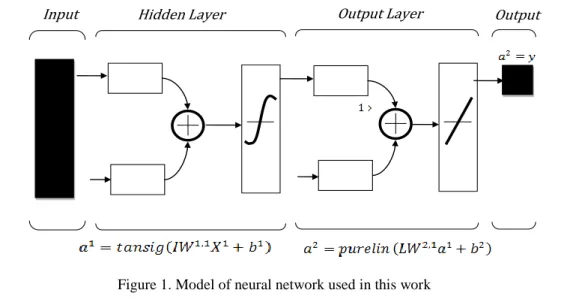
In fitting problems, a neural network map between a data set of numeric inputs and a set of numeric targets.The prediction of path loss is a fitting problem modeled as function approximation [9]. The neural network is expected to modify its weights and bias values in order to approximate the function relating the measured path loss values with the input variables (frequency of the transmitter, transmitting antenna height, receiving antenna height, distance from transmitting station, elevation of the receiving antenna, and the azimuth angle measured from the transmitter).The neural network is expected to take in a 6 input vector and produce a path loss estimate as its output. The architecture of a typical artificial neural network is shown in Figure 1.

Output Input

Hidden Layer Output Layer

Figure 1. Model of neural network used in this work

Large cities, fc ≤ 400MHz

Large cities, f

c ≥ 400MHz

(3)

This network can be used as a general function approximator. It can approximate any function with a finite number of discontinuities arbitrarily well, given sufficient neurons in the hidden layer [10]. The network depicted in Figure 1 above is a two layer feed-forward network with one hidden layer having tan sigmoid activation function and one output layer with linear activation function. A layer, as used in this work, is one that contains computational units i.e., it contains at least one neuron. A layer that produces the network output is called an output layer. All other layers are called hidden layers. In Figure 1, the layers are indicated with superscripts. Superscripts are used to identify the source (second index) and the destination (first index) for the various weights and other elements of the network. Here, weight matrices connected to inputs will be referred to as input weights; while weight matrices coming from layer outputs will be called layer weights. The weight matrix connected to the input vector x is labeled as an input weight matrix (IW1,1) having a source 1 (second index) and a destination 1 (first index). Elements of layer 1, such as its bias, net input, and output have a superscript 1 to indicate that they are associated with the first layer. The weight matrix connected to the hidden layer is labeled as a layer weight matrix (LW2,1) having a source 1 (second index) and a destination 2 (first index). The network shown in Figure 1 has 6 inputs, 7 neurons in the first layer, and oneneuron in the output layer. A constant input 1 is fed to the bias for each neuron. The input to layer 2 is a1; the output is a2. The output of the second layer a2, is the network output of interest, and this output is labeled as y. In this network, each element of the input vector x is connected to the input of each neuron in layer 1(hidden layer) through the input weight matrix IW. Each neuron has a summer that gathers its weighted inputs and bias to form its own scalar output n1. The various n1 taken together form a 5-element net input vector n1. The neuron layer outputs form a column vector a1. The expression for a1 is shown at the bottom of the Figure 1. The output vector a1 result after the tangent hyperbolic sigmoid activation function acts on the net input vector n1. The output vector a1from the hidden layer now serves as the input vector for the single neuron in the second layer (output layer). The neuron has a summer that gathers its weighted inputs and bias to form its own scalar output n2. The linear activation function for the output layer acts on n2 to produce the neuron output a2. The output a2 is the network output of interest and it is stored in the network output as y. In the network above, a non-linear differentiable activation function (or transfer function) was used due to its necessity for back-propagation. For the hidden layer, the tan sigmoid activation function was used. The linear output layer allows the network produce values outside the range -1 to +1. If sigmoid neurons are used in the output layer, then the outputs of the network are limited to a small range [10]Though feed-forward networks with more layers than the network in Figure 1 might be able to learn complex relationships more quickly, for the 422 data points used in this work, the two layer feed-forward network used had satisfactory training times.The input parameters for the ANN include the distance between transmitting station and receiving antenna in kilometers; operating frequency of transmitting station in mega hertz; the Elevation of the receiving antenna in feet; the azimuth angle from the transmitter to each receiving point in degrees; the height of the transmitting antenna; the height of the receiving antenna.Activation/Transfer function used is Hyperbolic tangent sigmoid function for the hidden layer and a linear transfer function for the output layer. A non linear transfer function was used in the hidden layer because of its differentiability, which is necessary for back propagation of errors. The hyperbolic tangent was used because the output could take positive or negative values. For the output layer, a linear function is used in place of a hard limiting or Heaviside function because it is a fitting or function approximation problem rather than a pattern recognition or classification one.

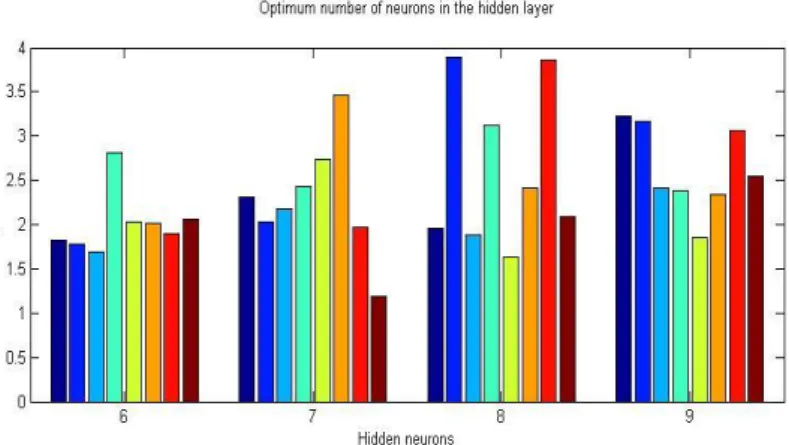
Number of hidden neurons: The actual number of hidden neurons was determined on the basis of trial and error [11]. Various random weight and bias initialization was done and number of hidden neurons was increased incrementally. The optimum number of hidden neurons was then determined by testing each iterated network on a sample data, and the network with the best performance, as indicated by the mean squared errors, was selected. This procedure helped to reduce the problem of local optima, through the various weight initializations, and also for selecting the optimum hidden neuron as measured by the mean squared error. Figure 2 shows bar graph showing optimization of hidden neurons.

The neural network with seven hidden neurons during the eighth random weight initialization was found to have the lowest mean square error of 1.1945. The Back-propagation network training function used is the Bayesian regularization. Bayesian regularization minimizes a linear combination of squared errors and weights. It also modifies the linear combination so that at the end of training the resulting network has good generalization qualities. Bayesian regularization describes a routine that automatically sets the regularization parameters [10]. The Back-propagation weight/bias learning function used is the Gradient descent with momentum for calculating the weight and bias changes. The momentum term is included in the standard gradient descent algorithm to improve the speed of learning and convergence [11]. To utilize Early Stopping, the training data is divided into two subsets (training and

(4)

validation_train; where validation_train is the validation data that is a subset of the training data) where the training set is used for computing the gradient and the ANN weights. The errors obtained from the validation set are monitored during the training. In this work, the number of input-output data pairs in the validation_train set is chosen to be 20% of the full training set. When the network is starting to over-fit the data from the training set, the errors obtained from the validation_train set usually start to increase. When the validation_train error has increased for a specified number of iterations the training stops and the weights and biases at the minimum of the validation error is returned.

Figure 2. Bar graph showing optimization of hidden neurons

The work presented in this study utilizes VHF/UHF radio wave propagation measurements at carrier frequencies of 189.25MHz, 479.25MHz, and 743.25MHz from three television broadcasting stations in Edo State, Nigeria. The measurements were conducted using a Field Strength Analyzer. The measurement system also includes a global positioning system (GPS) receiver and an omni-directional receiving antenna. The data originates from three television broadcasting transmitters taken from two different routes per transmitting station covering almost 80km of urban and sub-urban terrain per route. The heights of the transmitting stations were 137.16m, 304.8m, and 228.6m. The mobile receiving antenna height was 1.5m. A total amount of 422 data sets were collected covering three different UHF/VHF transmitters of various frequencies. Approximately 82 percent of the data sets were used for training the artificial neural network. The other 18 percent was split evenly into two parts and was used for validation. One of the validation set was used to select the optimum number of neurons in the hidden layer based on accurate generalization which was measured using mean squared error. The final validation set was used as an independent test of the performance of the neural network. Figure 3 shows pie chart showing division of dataset used in this paper.

Figure 3. Pie chart showing division of dataset used in this paper

3. Results and Analysis

After successful training and selection of the artificial neural network, the network was then used to predict the path loss of the test dataset. This data set was set aside, from the total pool of experimental data obtained, as an independent measure of the actual predictive ability of the network. This data was not used in the training or validation of the network. The statistical measures used to access the accuracy and

(5)

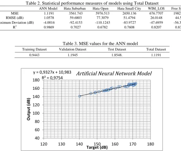
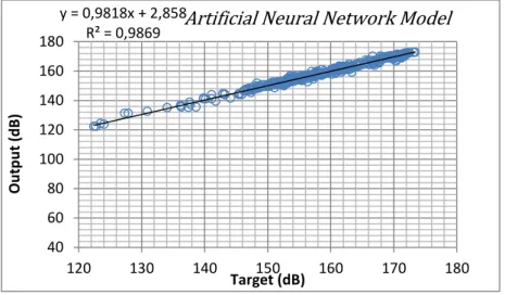
predictive ability of the neural networks and the empirical models used in this paper include; Mean Squared Error (MSE); Root mean square error or root mean square deviation (RMSE or RMSD), Maximum error Deviation, Coefficient of Determination (R-squared). Tables 1 and 2 show the computed values of the four statistical performance measures. These measures are for the artificial neural network and the empirical models used for comparison. Table 3 shows MSE values for the ANN model. Figure 4 shows regression plot for Artificial Neural Network Model using test data set. Figure 5 shows regression plot for Artificial Neural Network using total data set.

Table 1. Statistical performance measures of models using Test Dataset

ANN Model Hata Suburban Hata Open Hata Small City WIM_LOS Free Space MSE 1.8548 3520.1332 5958.6777 2567.2182 733.9782 2113.7778 RMSE (dB) 1.3619 59.33071 77.19247 50.66772 27.09203 45.97584 Maximum Deviation (dB) -3.4588 -89.1679 -107.4281 -79.7125 -48.1632 -56.4934 R2 _0.9754 _0.6751 _0.6465 _0.7425 _0.8627 _0.8808

Table 2. Statistical performance measures of models using Total Dataset

ANN Model Hata Suburban Hata Open Hata Small City WIM_LOS Free Space MSE 1.1191 3561.743 5976.513 2650.136 676.7707 1982.483 RMSE (dB) 1.0578 59.6803 77.3079 51.4794 26.0148 44.525 Maximum Deviation (dB) -4.0016 -92.4153 -110.1243 -83.9727 -47.6959 -56.3750

R2 _0.9869 _0.7027 _0.6782 _0.7608 _0.8207 _0.8373

Table 3. MSE values for the ANN model

Training Dataset Validation Dataset Test Dataset Total Dataset

0.9443 1.1945 1.8548. 1.1191

Figure 4. Regression plot for Artificial Neural NetworkModel using test data set

y = 0,9327x + 10,983 R² = 0,9754 40 60 80 100 120 140 160 180 120 130 140 150 160 170 180 Ou tp u t (d B ) Target (dB)

(6)

Figure 5. Regression plot for Artificial Neural Network using total data set

3.1. Discussion

The two datasets used for performance evaluation comprises the Test dataset and the Total dataset. The Test dataset was not used in training or validating the neural network. Hence, it serves as an independent sample for evaluating the neural network prediction performance for out of sample data that is completely new to it. Both the Total and Test datasets were used for comparison of the neural network with some selected empirical models. From Table 1, according to the all statistical measures used for performance evaluation, the ANN generally performed better for the test datasets compared to the Hata variants, the Walfisch-Ikegami Line of Sight, the free space models. For the mean squared errors, which generally incorporates both the bias and variance of the models, the ANN had an MSE of 1.8548 which was substantially smaller than that the other models. This shows that relatively, the ANN has a smaller variance and bias and is hence a better predictive model. For other measures, the ANN also performs better with an RMSE of only 1.3619dB and maximum error deviation of 3.4588. Using the R-squared from Table 1 as a statistical performance measure shows that the ANN with a value of 0.9754 explains most of the variability of the response data about the mean. In comparison with the other models in the table, the ANN model has a better fit for the response data and hence has a better predictive ability.

Table 2 shows the corresponding performance of the models when the entire experimental dataset is used. It is observed here that the MSE of the ANN is slightly better than that for the test dataset. This may be explained by the fact that the majority of the total dataset (82%) was used in training the network. And as such, the performance of the ANN is slightly biased for those datasets. As in the case of the test dataset the general performance trend still holds. It can be observed from Table 2 that the ANN still has better predictive ability in comparison with the selected empirical models as evidenced from its low MSE and RMSE values. Also, its r-squared value of 0.9869 shows that the ANN is an excellent estimator for path loss values in the VHF/UHF spectrum in Edo state.

The close correspondence of the ANN’s output with the experimentally determined path loss values can be clearly seen in the path loss plots for the three television transmitting stations along the Ekpoma route shown in Figures 6 to 8. As observed from Figures 6 to 8 and from the maximum deviation value in Tables 1 and 2 that all the empirical models under-predict the path loss values for all environments and for the test and total datasets.

y = 0,9818x + 2,858 R² = 0,9869 40 60 80 100 120 140 160 180 120 130 140 150 160 170 180 Ou tp u t (d B ) Target (dB)

(7)

Figure 6. Path loss for ITV Benin along Ekpoma route, 479.25MHz

Figure 7. Path loss for NTA Benin along Ekpoma route, 189.25MHz

Figure 8. Path loss for EBS along Ekpoma route, 743.25MHz

40 60 80 100 120 140 160 0 10 20 30 40 50 60 70 80 90 Path Lo ss (d B ) Distance (KM) Hata Subur ban Hata Open Hata Small

Path loss plot showing predictive models for ITV Benin along Ekpoma route,

40 60 80 100 120 140 160 0 20 40 60 80 Path Lo ss (d B ) Distance (KM) Hata Suburb an Hata Open Hata Small WIM_L OS

Path loss plot showing predictive models for NTA Benin along Ekpoma route, 189.25MHz

40 60 80 100 120 140 160 180 0 20 40 60 80 Path Lo ss (d B ) Distance (KM) Hata Large Hata Suburba n Hata Open Hata Small

(8)

4. Conclusion

A neural network approach to the prediction of path loss in UHF/VHF signal propagation In Edo state was considered. The basic Idea is to yield path loss prediction using the ANN network, by first training it with data obtained experimentally. It is essential that the training data should be of similar profile to the dataset that the neural network is required to predict. The artificial neural network designed in this paper (with two feed-forward layers, having a tan sigmoid hidden layer and a linear output layer) had high performance with predicting path loss values in the VHF/UHF frequency spectrum in Edo state. The neural network produced had high accuracy when both training and non-training data was used. The neural network had a slightly better accuracy for training dataset as compared to non- training datasets. This was estimated using the mean square error and r-squared values. Especially useful was that the network generalized well with independent data from the test dataset. The neural network was found out to be a better estimator of path loss values for signal propagation in the VHF/UHF band in Edo State as compared with traditional empirical path loss models like the Hata and Walfisch-Ikegami line of sight models. To improve the robustness of the neural network design, very large and varied measurement data, which contains knowledge of different environmental profiles, should be used to train the network.

Acknoledgements

The authors wish to appreciate the management of the university of Benin for grant given which contributed to this work

References

[1] H. Bertoni, “Coverage prediction for mobile radio systems operating in the 800/900 MHz frequency range,”

IEEE Transactions on Vehicular Technology, vol. 37, no. 1, pp. 3–72, February 1988.

[2] C. A. Zelley and C. C. Constantinou, “A three-dimensional parabolic equation applied to VHF/UHF propagation

over irregular terrain,” IEEE Transactions on Antennas and Propagation, vol. 47, no. 10, pp. 1586–1596,

October 1999.

[3] E. Ostlin, et al “In press:Macrocell radio wave propagation prediction using an artificial neural network,” IEEE

Transactions on Vehicular Technology, 2010

[4] K. E. Stocker and F. M. Landstorfer, “Empirical prediction of radiowave propagation by neural network

simulator,” Electronics Letters, vol. 28, no. 12, pp. 1177–1178, June 1992

[5] I. Popescu, et al, “ANN prediction models for outdoor environment,” in 17th IEEE International Symposium on

Personal, Indoor and Mobile Radio Communications, Helsinki, Finland, pp. 1–5, September 2006.

[6] Z. Stankovi et al , “The hybrid-neural empirical model for the electromagnetic field level prediction in urban

environments,” in 7th Seminar on Neural Network Applications in Electrical Engineering, Belgrade, Serbia, pp. 189–192, September 2004.

[7] A. Neˇsković, N. Neˇsković, and D. Paunović, “Indoor electric field level prediction model based on the

artificial neural networks,” IEEE Communications Letters, vol. 4, no. 6, pp. 190–192, June 2000.

[8] Walter Debus, “RF Path Loss & Transmission Distance Calculations,” Axonn, LLC, Technical Memorandum,

August 4, 2006.

[9] M.H. Beale, Martin T. Hagan, Howard B. Demuth, “Neural Network Toolbox™ User’s Guide R2013a,”

MathWorks, Inc., 2013.

[10] H.Simon, “Neural networks: A comprehensive foundation,” Prentice Hall International, Inc., Second

Edition, 1999.

[11] Ning Qian,”Contributed Article On the momentum term in gradient descent learning algorithms,” Center for

Neurobiology and Behavior, Columbia University, New York, USA Neural Networks vol. 12, pp. 145–151, 1999.