213
© Global Society of Scientific Research and Researchers
http://asrjetsjournal.org/
An Improvement to LMSV Parameter Estimation:
Modelling and Forecasting Volatility and Value-at-risk
Grace Lee Ching Yap
a*, Wen Cheong Chin
ba
School of Applied Mathematics, Faculty of Engineering, (Malaysia Campus), 43500 Semenyih, Selangor, Malaysia
b
Faculty of Management, SIG Quantitative Economics and Finance, Multimedia University, 63100 Cyberjaya, Selangor, Malaysia a Email: [email protected] b Email: [email protected] Abstract
This paper proposes an improvement to the long memory stochastic volatility (LMSV) model to forecast volatility using high frequency data. To allow frequency domain quasi-maximum likelihood (FDQML) estimation, we suggest a parsimonious normalization procedure that avoids repetitive parameter estimation. This resultantly produces more efficient parameter estimation as less estimation error is involved. Besides, a de-trending procedure is proposed prior to the de-seasonalization procedure to improve the identification of seasonal patterns. We compare the performance of volatility forecasts by the proposed refined FDQML-LMSV model with the existing LMSV and the linear long memory model that fits to logarithms of realised volatility. The empirical results show that the proposed method outperforms the existing models statistically, and the output of the proposed method improves the accuracy and efficiency in value-at-risk forecasting.
Keywords: long memory; volatility; normalization; value-at-risk.
1.Introduction
The availability of vast high-frequency data on returns of financial assets has spurred an enormous research in the modelling and forecasting of return volatility.
--- * Corresponding author.
214
Particularly, realized volatility (RV) which can be easily computed from high-frequency intra-day returns is introduced and promoted by [1–3]. The superiority of RV as an efficient estimator of return volatility is supported by the subsequent work of [4–6], which showed that RV modelled with autoregressive fractionally integrated moving average (ARFIMA) generally performs better than ARCH models for volatility forecasting. The significance of reliable volatility predictions is seen in the estimate and forecast of value-at-risk (VaR), the most sought-after technique that has been vigorously studied in quantitative risk management and financial econometrics. Several authors demonstrated that an accurately predicted volatility is materialized into economic benefits in the context of VaR forecasting [7–9].
RV is obtained by aggregating the high-frequency squared returns over a desired estimation or forecast horizon. Noting that RV has long memory property and high-frequency returns exhibit seasonality in volatility, Deo and his colleagues [10] proposed a time varying de-seasonalization method within the long memory stochastic volatility (LMSV) model. The LMSV model is suitable for financial returns that are captured at equally spaced time interval. To estimate the parameters of the LMSV model, the authors followed the frequency domain quasi maximum likelihood (FDQML) method which assumes a Gaussian time series. A power transformation to the series was suggested to meet such assumption. This approach is rather laborious because besides searching for a power that transforms the series into a Gaussian time series, it also requires the estimation of the spectral density and the covariance matrix of the transformed series as there is no analytic spectral density available for the powered transformed series. There are other models proven to be able to capture the long memory of the volatility such as heterogeneous autoregressive [11] and autoregressive fractionally integrated model [12]. The authors compared the performance of their FDQML-LMSV models with that of linear long-memory models fit to log RV proposed by Andersen and his colleagues [12] (ABDL). It was reported that the ABDL method is a very good competitor to Deo’s FDQML-LMSV models, especially when forecasting over a short horizon.
On the other hand, it has become increasingly clear that economic and financial series contain cyclical component [13,14]. As such, it is necessary to pre-treat a financial time series with an elimination of cyclical and seasonality components before it is transformed into a Gaussian time series. In the data pre-treatment procedure, prior to Deo’s time varying de-seasonalization, we propose a trend elimination adjustment in the form of linear combination of a sine and a cosine evaluated at Fourier frequencies in multiple of an appropriate number of periods per cycle. Besides the trend elimination, this paper also contributes to improve the FDQML-LMSV model in the aspect of normalization and the back-transformation procedures. The normalization procedure is rather simple as it only involves fitting the empirical cumulative probabilities to the Gaussian cumulative distribution function [15]. For the purpose of back-transformation, a Weibull distribution is used to model the empirical data so that a normal cumulative probability can be matched to a point within the distribution of the pre-processed data. Nonetheless, a convex transformation is involved to recover the forecast of RV from log RV. To close down the gap of difference, we propose an adjustment factor that takes the overall weights of the linear combination in the forecast equation.
Although ABDL reported that the distributions of the logarithms of realized volatilities are approximately Gaussian, it is interesting to know if the proposed normalization procedure improves the ABDL model. The proposed improvement to the FDQML-LMSV and the ABDL models are estimated and used to forecast realized
215
volatility at various horizons for S&P500 and DAX indices. Besides, as the volatility forecastability is relevant for short time horizons, we evaluate the forecasts economically via their VaR performance for daily trading made up of long and short positions. It is found that the proposed procedures to FDQML-LMSV and ABDL models improve the accuracy in the RV forecasts and hence produce VaR forecasts with capital efficiency.
The rest of the paper is organized as follows. Section 2 describes the FDQML-LMSV model. Section 3 presents the enhancement to FDQML-LMSV model. Section 4 presents the empirical analysis using the proposed methodology for statistical and economic forecast evaluations, and finally Section 5 concludes.
2. FDQML-LMSV model
The LMSV model for the returns 𝑟𝑟𝑡𝑡,𝑡𝑡= 1, … ,𝑛𝑛 is given by
𝑟𝑟𝑡𝑡=𝜎𝜎exp�ℎ2𝑡𝑡� 𝜀𝜀𝑡𝑡 (1)
Where 𝜀𝜀𝑡𝑡 ~ 𝑖𝑖𝑖𝑖𝑖𝑖(0, 1), 𝜎𝜎> 0 and {ℎ𝑡𝑡} is a stationary zero mean Gaussian long-memory process independent of
{𝜀𝜀𝑡𝑡}. For the sake of simplicity, we assume that {ℎ𝑡𝑡} follows an autoregressive fractionally integrated moving
average ARFIMA (𝑝𝑝,𝑖𝑖,𝑞𝑞) that takes the form Φ(𝐿𝐿)(1− 𝐿𝐿)𝑑𝑑ℎ𝑡𝑡=Θ(𝐿𝐿)𝜂𝜂𝑡𝑡, where 𝐿𝐿 is the backshift operator, 𝜂𝜂𝑡𝑡 ~𝑖𝑖𝑖𝑖𝑖𝑖𝑁𝑁�0,𝜎𝜎𝜂𝜂2�, 0 <𝑖𝑖< 0.5,Φ(𝐿𝐿) and Θ(𝐿𝐿) are polynomials of orders 𝑝𝑝 and 𝑞𝑞 with all roots outside the unit
circle. Prior to forecasting with the LMSV model, Deo and his colleagues [10] reasoned that it is necessary to eliminate the seasonal component in volatility, which shows periodic peaks in the periodogram of the log squared returns. The authors proposed a time varying seasonal adjustment procedure in the form of
𝑅𝑅𝑡𝑡= exp�𝑆𝑆2𝑡𝑡� 𝑟𝑟𝑡𝑡 (2)
where 𝑅𝑅𝑡𝑡 is the high frequency return demeaned by sample mean 𝜇𝜇̂𝑅𝑅, 𝑆𝑆𝑡𝑡 is the seasonal component and 𝑟𝑟𝑡𝑡 is the de-seasonalized high frequency return. The seasonality is written as a linear combination of sines and cosines evaluated at the Fourier frequencies with seasonal peaks as follows:
𝑆𝑆𝑡𝑡=� 𝑎𝑎𝑝𝑝𝑐𝑐𝑐𝑐𝑐𝑐 𝜔𝜔𝑝𝑝𝑡𝑡 𝑘𝑘 𝑝𝑝=1 +� 𝑏𝑏𝑝𝑝𝑐𝑐𝑖𝑖𝑛𝑛 𝜔𝜔𝑝𝑝𝑡𝑡 𝑘𝑘 𝑝𝑝=1 (3)
where {𝜔𝜔𝑝𝑝}𝑝𝑝=1𝑘𝑘 is the collection of Fourier frequencies at the seasonal peaks and their neighbouring frequencies that exhibit large magnitudes. The coefficients 𝑎𝑎𝑝𝑝 and 𝑏𝑏𝑝𝑝 can be obtained by running an equivalent regression
log𝑅𝑅𝑡𝑡2=∑𝑘𝑘𝑝𝑝=1𝑎𝑎𝑝𝑝cos𝜔𝜔𝑝𝑝𝑡𝑡+∑𝑘𝑘𝑝𝑝=1𝑏𝑏𝑝𝑝sin𝜔𝜔𝑝𝑝𝑡𝑡+𝑒𝑒𝑡𝑡where 𝑒𝑒𝑡𝑡 is the residual term.
In the FDQML estimation procedure, the log squared de-seasonalized returns are expressed as a sum of a Gaussian long-memory signal plus a zero mean noise series, i.e., 𝑍𝑍𝑡𝑡= log(𝑟𝑟𝑡𝑡2) =𝜇𝜇+ℎ𝑡𝑡+𝜉𝜉𝑡𝑡 where 𝜉𝜉𝑡𝑡=
216 𝑓𝑓�𝜔𝜔𝑗𝑗�=𝜎𝜎𝜂𝜂 2 2𝜋𝜋 �𝛩𝛩�−𝑖𝑖𝜔𝜔𝑗𝑗��2 �𝛷𝛷�−𝑖𝑖𝜔𝜔𝑗𝑗��2�1− 𝑒𝑒𝑒𝑒𝑝𝑝�−𝑖𝑖𝜔𝜔𝑗𝑗��2𝑑𝑑 +𝜎𝜎2𝜉𝜉𝜋𝜋2 (4)
where 𝜎𝜎𝜉𝜉2 is the variance of 𝜉𝜉𝑡𝑡. The parameters are estimated by minimizing the Whittle approximation given below: ℒ= � �𝑙𝑙𝑐𝑐𝑙𝑙 �𝑓𝑓�𝜔𝜔𝑗𝑗��+𝑓𝑓�𝜔𝜔𝐼𝐼𝑗𝑗 𝑗𝑗�� �𝑛𝑛−12 � 𝑗𝑗=1 (5) where 𝐼𝐼𝑗𝑗= 1 2𝜋𝜋𝑛𝑛�∑𝑛𝑛𝑡𝑡=1𝑍𝑍𝑡𝑡exp�−𝑖𝑖𝜔𝜔𝑗𝑗�� 2
is the periodogram of 𝑍𝑍𝑡𝑡 at the 𝑗𝑗𝑡𝑡ℎFourier frequency 𝜔𝜔𝑗𝑗=2𝜋𝜋𝑗𝑗
𝑛𝑛 , and [∙] is
the integer part of (∙).
Deo and his colleagues [10] argued that 𝑍𝑍𝑡𝑡 is not Gaussian, and hence, a transformed series |𝑟𝑟𝑡𝑡|𝑐𝑐 was suggested of which 𝑐𝑐 is chosen such that the transformed series is closer to Gaussian than that of log(𝑟𝑟𝑡𝑡2). This is done by setting the skewness of |𝑟𝑟𝑡𝑡|𝑐𝑐 to zero based on the initial parameter estimates of the LMSV model on log(𝑟𝑟𝑡𝑡2). Although the power transformation can be done quite easily to meet the assumption of normality, it is noted that the transformed series does not have the spectral density as given in Eq.(4), and hence, the Whittle approximation cannot be applied straightaway. Based on bivariate expected values and the initial parameter estimates of the LMSV model on log(𝑟𝑟𝑡𝑡2), the authors suggested that the spectral density of |𝑟𝑟𝑡𝑡|𝑐𝑐 is to be estimated from its auto-covariance function via Fourier transform. Subsequently, the FDQML estimation for series |𝑟𝑟𝑡𝑡|𝑐𝑐 is done by using the Whittle likelihood in Eq. (5), with 𝑓𝑓 and 𝐼𝐼 being the spectral density and the periodogram of |𝑟𝑟𝑡𝑡|𝑐𝑐respectively. Once the parameters are estimated, the one-step ahead realized volatility forecast can be computed based on the best linear predictor below.
E�rn+12 − µr,2− �Aj∗ ��rn−j�c− µr,c� n−1
j=0
�
2 (6)
where 𝜇𝜇𝑟𝑟,2=𝐸𝐸(𝑟𝑟𝑡𝑡2), 𝜇𝜇𝑟𝑟,𝑐𝑐 =𝐸𝐸(|𝑟𝑟𝑡𝑡|𝑐𝑐), and the coefficients 𝐴𝐴𝑗𝑗 are the solution set of the linear equations given by
𝐄𝐄𝐂𝐂𝐀𝐀=γ2,c,1 (7)
where 𝑬𝑬𝒄𝒄=𝑐𝑐𝑐𝑐𝑐𝑐(|𝑟𝑟𝑛𝑛|𝑐𝑐,⋯, |𝑟𝑟1|𝑐𝑐),𝛾𝛾2,𝑐𝑐,1= [𝑐𝑐𝑐𝑐𝑐𝑐(𝑟𝑟𝑛𝑛+12 , |𝑟𝑟𝑛𝑛|𝑐𝑐),⋯,𝑐𝑐𝑐𝑐𝑐𝑐(𝑟𝑟𝑛𝑛+12 , |𝑟𝑟1|𝑐𝑐)]′, and 𝑨𝑨= (𝐴𝐴0,⋯,𝐴𝐴𝑛𝑛−1 )′. The entries of 𝑬𝑬𝒄𝒄and 𝛾𝛾2,𝑐𝑐,1 are obtained using bivariate expected values that rely on the parameters of the LMSV model on |𝑟𝑟𝑡𝑡|𝑐𝑐. The best one-step ahead linear predictor of 𝑟𝑟𝑛𝑛+12 is then given by
r
�n+12 =µr,2+�Aj∗ ��rn−j�c− µr,c� n−1
j=0
(8)
217
returns 𝑟𝑟̂𝑛𝑛+12 using Eq.(8) may not be optimal as squared returns are not Gaussian. They proposed another method, called LMSVc to counter this problem. LMSVc is different from LMSV2 such that the best linear forecast, say |𝑟𝑟̂𝑛𝑛+1|𝑐𝑐, of |𝑟𝑟𝑛𝑛+1|𝑐𝑐 is predicted based on |𝑟𝑟𝑛𝑛|𝑐𝑐, … , |𝑟𝑟1|𝑐𝑐. The forecast of 𝑟𝑟𝑛𝑛+12 is obtained by using power transformation 𝑟𝑟̂𝑛𝑛+12 =𝐸𝐸 �|𝑋𝑋|𝑐𝑐2�, where 𝑋𝑋 is a normal random variable with mean |𝑟𝑟̂𝑛𝑛+1|𝑐𝑐 and variance
𝜎𝜎𝑐𝑐2,1=𝐸𝐸(|𝑟𝑟𝑛𝑛+1|𝑐𝑐−|𝑟𝑟̂𝑛𝑛+1|𝑐𝑐)2. Assume that a high-frequency data set contains 𝑚𝑚 intra-day returns in a trading
day such that the forecast of the RV for the next trading day depends on the forecasts {𝑟𝑟̂𝑛𝑛+12 ,⋯,𝑟𝑟̂𝑛𝑛+𝑚𝑚2 }. These squared return forecasts are obtained by repeating Eq.(8) 𝑚𝑚 times, of which in each iteration-𝑖𝑖,𝑖𝑖= 2, … ,𝑚𝑚, the most recent past observation |𝑟𝑟𝑛𝑛+𝑖𝑖−1|𝑐𝑐is updated with the forecast that has just been generated |𝑟𝑟̂𝑛𝑛+𝑖𝑖−1|𝑐𝑐. Subsequently, the forecasts of squared returns are re-seasonalized to give {𝑅𝑅�𝑡𝑡2}𝑡𝑡=𝑛𝑛+1𝑛𝑛+𝑚𝑚 , and the RV for the next trading day is predicted as the sum of these 𝑚𝑚 intra-day squared returns 𝑅𝑅𝑅𝑅��𝑛𝑛
𝑚𝑚�+1=∑ 𝑅𝑅�𝑡𝑡
2 𝑛𝑛+𝑚𝑚
𝑡𝑡=𝑛𝑛+1 .
Despite thorough considerations given to LMSV model, it is outperformed by a simple ARFIMA(1,𝑖𝑖,0) model applied to log𝑅𝑅𝑅𝑅, especially when forecasting over a short horizon. This can be due to the noise generated when the power 𝑐𝑐 is determined based on the initial parameter estimates of the LMSV model on log(𝑟𝑟𝑡𝑡2). Besides, it is good to examine if there is other information contained in log𝑅𝑅𝑡𝑡2other than the time varying seasons so that 𝑍𝑍𝑡𝑡 truly represents a sum of a Gaussian long-memory signal plus a zero mean noise series. To address these concerns, we suggest the improvement in the following section.
3. Refined FDQML-LMSV model
Besides seasonality, a financial time series may contain cyclical trend. A graphical inspection of the time series plot is sufficient to determine the number of cycles per period. Similar to the approach of modelling the cyclical trend in [14], we suggest to estimate the trend component at cyclical frequencies. Based on the number of cycles per period, say 𝑘𝑘, observed in the time series plot, the trend component is fitted as a linear combination of a sine and a cosine evaluated at the Fourier frequencies in multiple of 𝑘𝑘, defined as follows:
TLRj=α𝑐𝑐𝑖𝑖𝑛𝑛 �ωn
kj�+β 𝑐𝑐𝑐𝑐𝑐𝑐 �ωnkj�+ c, j = 0, 1. … , n−1
(9)
where 𝜔𝜔𝑛𝑛
𝑘𝑘𝑗𝑗 are the Fourier frequencies with indices that are integer multiples of 𝑘𝑘. The coefficients 𝛼𝛼,𝛽𝛽 and the
constant 𝑐𝑐 are estimated using the least squares method within the curve fitting procedure in Matlab.
To identify the seasonal pattern efficiently, the cyclical trend in the log squared returns is to be eliminated and the de-trended series is obtained as 𝑟𝑟𝑒𝑒𝑐𝑐𝐿𝐿𝑅𝑅𝑡𝑡= log𝑅𝑅𝑡𝑡2− 𝑇𝑇𝐿𝐿𝑅𝑅𝑡𝑡−1. 𝑟𝑟𝑒𝑒𝑐𝑐𝐿𝐿𝑅𝑅𝑡𝑡 is then de-seasonalized following Deo’s time varying seasonalization procedure as described in Section 2. Let’s denote the trended and de-seasonalized series as log𝑟𝑟𝑡𝑡2∗. It is shown in Section 4 that these pre-processing steps can effectively eliminate the effects of trends and seasons, and hence, preparing the data suitable for the LMSV modelling.
After these pre-processing procedures, we propose to normalize log𝑟𝑟𝑡𝑡2∗ based on a comparison between the empirical and Gaussian cumulative distributions. This procedure is adopted from [15] whereby the normal
218
variate 𝑧𝑧𝑡𝑡 is produced by matching the cumulative probability 𝑃𝑃�log𝑟𝑟𝑡𝑡2∗� to the Gaussian cumulative distribution 𝐷𝐷(𝑧𝑧𝑡𝑡) with the mean 𝑧𝑧̅=𝐸𝐸(log𝑟𝑟𝑡𝑡2∗) and the variance 𝜎𝜎𝑧𝑧2=𝐸𝐸 �log𝑟𝑟𝑡𝑡2∗− 𝐸𝐸�log𝑟𝑟𝑡𝑡2∗��
2 as follows: D(zt) = 1 σz√2π� 𝑒𝑒𝑒𝑒𝑝𝑝 � (x−z�)2 2σz2 �dx zt −∞ = P(𝑙𝑙𝑐𝑐𝑙𝑙rt ∗ 2) (10)
The normality of series {𝑧𝑧𝑡𝑡} can be verified by using Jarque-Bera test. It is noted that the transformed series {𝑧𝑧𝑡𝑡} has the spectral density in the form of Eq.(4), which permits the application of Whittle approximation in Eq.(5). Subsequently, the one-step ahead normalized log squared return, 𝑧𝑧𝑛𝑛+1, is computed similar to the best linear predictor in Eq.(8), except that the series {|𝑟𝑟𝑡𝑡|𝑐𝑐} is replaced by {𝑧𝑧𝑡𝑡}, and the expected value as well as the auto-covariance are computed based on {𝑧𝑧𝑡𝑡} and its respective LMSV parameters as shown below.
z
�n+1=µz+�Aj∗(zn−j− µz) n−1
j=0
(11)
where 𝜇𝜇𝑧𝑧=𝐸𝐸(𝑧𝑧𝑡𝑡), and 𝐴𝐴𝑗𝑗 are the coefficients in Eq.(7) with 𝑬𝑬𝒄𝒄and 𝛾𝛾2,𝑐𝑐,1 being replaced by 𝑐𝑐𝑐𝑐𝑐𝑐(𝑧𝑧𝑛𝑛,⋯,𝑧𝑧1) and
[𝑐𝑐𝑐𝑐𝑐𝑐(𝑧𝑧𝑛𝑛+1,𝑧𝑧𝑛𝑛),⋯,𝑐𝑐𝑐𝑐𝑐𝑐(𝑧𝑧𝑛𝑛+1,𝑧𝑧1)]′ respectively. The one-step ahead forecast 𝑧𝑧̂𝑛𝑛+1has to be back-transformed to
be of any utility. This requires the distributional form of log𝑟𝑟𝑡𝑡2∗. To do this, we fit the probability distribution of
log𝑟𝑟𝑡𝑡2∗ with Weibull distribution due to its flexibility to assume various characteristics. In fact, Weibull distribution is popular amongst the quality practitioners in survival analysis, reliability engineering, hydrology as well as weather forecasting [15]–[18]. The Weibull probability density function is given below:
f(yt) =ba�yat� b−1
𝑒𝑒𝑒𝑒𝑝𝑝 �− �yat�b�, yt≥0
(12)
where 𝑎𝑎 and 𝑏𝑏 are the scale and shape parameters to be estimated using maximum likelihood estimates given the values in the series {𝑦𝑦𝑡𝑡}. To ensure that 𝑦𝑦𝑡𝑡≥0, we suggest that the de-trended and de-seasonalized series
log𝑟𝑟𝑡𝑡2∗ is to be adjusted such that 𝑦𝑦𝑡𝑡= log𝑟𝑟𝑡𝑡2∗− 𝑦𝑦m∗ + 0.1, where 𝑦𝑦m∗ is the minimum of {log𝑟𝑟𝑡𝑡2∗}. With this
distributional form, the forecast 𝑧𝑧̂𝑛𝑛+1can be connected to log𝑟𝑟̂(2𝑛𝑛+1)∗ in two steps. First, the Gaussian cumulative distribution function 𝐷𝐷(𝑧𝑧̂𝑛𝑛+1) is matched to the Weibull cumulative distribution function 𝐹𝐹𝑤𝑤(𝑦𝑦�𝑛𝑛+1) = 1−
exp�− �𝑦𝑦�𝑛𝑛+1 𝑎𝑎 �
𝑏𝑏
�, such that 𝐷𝐷(𝑧𝑧̂𝑛𝑛+1) =𝐹𝐹𝑤𝑤(𝑦𝑦�𝑛𝑛+1). Next, the forecast is adjusted back to its original scale, that is
log𝑟𝑟̂(2𝑛𝑛+1)∗=𝑦𝑦�𝑛𝑛+1+𝑦𝑦m∗ −0.1.
We follow the one-step-ahead forecast procedure as outlined in Section 2, whereby 𝑚𝑚 one-step ahead forecast �𝑟𝑟̂(2𝑛𝑛+1)∗,⋯ ,𝑟𝑟̂(2𝑛𝑛+𝑚𝑚)∗� are taken to form the next daily forecast 𝑅𝑅𝑅𝑅��𝑚𝑚𝑛𝑛�+1. From Eq.(11), we note that the forecast
𝑧𝑧̂𝑛𝑛+1 relies heavily on the linear combination of the past values {𝑧𝑧𝑛𝑛,𝑧𝑧𝑛𝑛−1,⋯,𝑧𝑧1} that can be matched to
{log𝑟𝑟𝑛𝑛2∗, log𝑟𝑟(2𝑛𝑛−1)∗⋯, log𝑟𝑟12∗}. Focusing on the linear combination, we have
219
𝑧𝑧̂𝑛𝑛+2≈ 𝐴𝐴0𝑧𝑧̂𝑛𝑛+1+𝐴𝐴1𝑧𝑧𝑛𝑛+ ⋯+𝐴𝐴𝑛𝑛−1𝑧𝑧2
⋮
𝑧𝑧̂𝑛𝑛+𝑚𝑚 ≈ 𝐴𝐴0𝑧𝑧̂𝑛𝑛+𝑚𝑚−1+𝐴𝐴1𝑧𝑧̂𝑛𝑛+𝑚𝑚−2+ ⋯+𝐴𝐴𝑛𝑛−1𝑧𝑧𝑚𝑚
According to Jensen’s inequality, we anticipate that exp�log𝑟𝑟̂(2𝑛𝑛+𝑗𝑗)∗�<𝑟𝑟(2𝑛𝑛+𝑗𝑗)∗,𝑗𝑗= 1,⋯,𝑚𝑚, of which
exp�log𝑟𝑟̂(2𝑛𝑛+𝑗𝑗)∗� can be matched to exp�𝑧𝑧̂𝑛𝑛+𝑗𝑗� ≈exp�𝐴𝐴0𝑧𝑧̂𝑛𝑛+𝑗𝑗−1+𝐴𝐴1𝑧𝑧̂𝑛𝑛+𝑗𝑗−2+ ⋯+𝐴𝐴𝑛𝑛−1𝑧𝑧𝑗𝑗�. To adjust the error due to the convex transformation, we propose to consider an average effect across the 𝑚𝑚 one-step-ahead forecasts. With this notion, let us estimate the linear combination as a product of the mean 𝑧𝑧̅=𝐸𝐸(log𝑟𝑟𝑡𝑡2∗) and the sum of coefficients 𝐴𝐴𝑗𝑗. As these forecasts are obtained based on the observation sets that are updated with the preceding forecasts, the sum of coefficients of each one-step ahead forecast can be explained as follows:
forecast sum of coefficients
z �n+1 s1=∑n−1j=0 Aj z �n+2 s2= A0∗s1+∑n−1j=1 Aj ⋮ ⋮ z�n+m sm= A0∗sm−1+⋯+ Am−2∗s1+ � Aj n−1 j=m−1
We propose to adjust the difference in exp�log𝑟𝑟̂(2𝑛𝑛+𝑗𝑗)∗� and 𝑟𝑟(2𝑛𝑛+𝑗𝑗)∗,𝑗𝑗= 1,⋯,𝑚𝑚, by multiplying a constant 𝑐𝑐𝑤𝑤 to the forecast exp�log𝑟𝑟̂(2𝑛𝑛+𝑗𝑗)∗�,𝑗𝑗= 1,⋯,𝑚𝑚. The constant 𝑐𝑐𝑤𝑤 is a ratio that corrects the effect of convex transformation given as follows:
cw=E(𝑒𝑒𝑒𝑒𝑝𝑝(κ ∗{zt}t=1
n ))
𝑒𝑒𝑒𝑒𝑝𝑝(κ ∗z�)
(13)
Where 𝜅𝜅 is the average of 𝑐𝑐𝑖𝑖,𝑖𝑖= 1,⋯ 𝑚𝑚.
In short, the forecast of the pre-processed squared return is obtained by
r
�(2n+j)∗=𝑒𝑒𝑒𝑒𝑝𝑝�Fw−1(D(z�n+j)) + y𝑚𝑚∗ −0.1� ∗cw, j = 1, … , m (14)
where 𝐹𝐹𝑤𝑤−1(∙) is the inverse Weibull cumulative distribution function.
The forecast of the squared returns 𝑅𝑅�𝑛𝑛+𝑗𝑗2 is subsequently obtained after the procedures to undo the de-seasonalization, mean and trend adjustments. We follow Deo’s procedures to re-seasonalize the returns. To undo the trend adjustment, the forecast 𝑟𝑟̂(2𝑛𝑛+𝑗𝑗)∗ is added back with 𝑇𝑇𝐿𝐿𝑅𝑅� 𝑛𝑛+𝑗𝑗 following Eq.(9), where the argument is 𝜔𝜔�𝑛𝑛
𝑘𝑘(𝑛𝑛+𝑗𝑗) = 2𝜋𝜋𝑘𝑘
220 R �2n+j=��𝑒𝑒𝑒𝑒𝑝𝑝�S n+j−m+ TLR� n+j� ∗r�(2n+j)∗+µ�R� 2 , j = 1,⋯, m (15)
where 𝜇𝜇̂𝑅𝑅 is the sample mean of {𝑅𝑅𝑡𝑡} 𝑡𝑡=1𝑛𝑛 .
The RV for the next trading day is predicted as the sum of squared returns, that is 𝑅𝑅𝑅𝑅��𝑛𝑛
𝑚𝑚�+1=∑ 𝑅𝑅�𝑡𝑡
2 𝑛𝑛+𝑚𝑚
𝑡𝑡=𝑛𝑛+1 .
In short, the refined FDQML-LMSV procedures can be summarized as follows, with steps (2), (4), (8) and (9) being the proposed enhancement. Let the first estimation window be {𝑅𝑅𝑡𝑡2}𝑡𝑡=1𝑛𝑛 , and assume that the observations
{𝑅𝑅𝑡𝑡2}𝑡𝑡=1𝑛𝑛+𝑚𝑚∗𝑖𝑖are available after �𝑚𝑚𝑛𝑛�+𝑖𝑖 – day of forecast. To obtain the forecast 𝑅𝑅𝑅𝑅��𝑛𝑛 𝑚𝑚�+𝑖𝑖:
(1) Obtain a demeaned log returned squared series log𝑅𝑅𝑡𝑡2− 𝜇𝜇̂. (2) Perform de-trending using Eq.(9). Get 𝑟𝑟𝑒𝑒𝑐𝑐𝐿𝐿𝑅𝑅𝑡𝑡.
(3) Perform de-seasonalization on 𝑟𝑟𝑒𝑒𝑐𝑐𝐿𝐿𝑅𝑅𝑡𝑡using Eq.(3). This gives log𝑟𝑟𝑡𝑡2∗. (4) Perform normalization using Eq.(10). This gives 𝑧𝑧𝑡𝑡.
(5) Estimate the LMSV parameters based on 𝑧𝑧𝑡𝑡.
(6) Estimate the covariance function of 𝑧𝑧𝑡𝑡 based on an assumed ARFIMA model. (7) Perform one-step-ahead forecast 𝑧𝑧̂𝑛𝑛+𝑗𝑗,𝑗𝑗= 1, … ,𝑚𝑚 using linear predictor in Eq.(11).
(8) Obtain the parameters of the Weibull fit to log𝑟𝑟𝑡𝑡2∗ distribution using Eq.(12). Take note of the adjustment for positive input.
(9) Obtain the forecast of the pre-processed squared return 𝑟𝑟̂(2𝑛𝑛+𝑗𝑗)∗using Eq.(14). (10)Obtain the forecast of the squared return 𝑅𝑅�𝑛𝑛+𝑗𝑗2 using Eq.(15).
(11)Compute the forecast 𝑅𝑅𝑅𝑅��𝑛𝑛
𝑚𝑚�+𝑖𝑖 using the results from step (10).
(12)Next estimation window is {𝑅𝑅𝑡𝑡2}𝑡𝑡=1+𝑚𝑚∗𝑖𝑖𝑛𝑛+𝑚𝑚∗𝑖𝑖 .
Repeat steps (1) – (12) until all the out-of-sample forecasts are sought. It can be seen that the proposed method is less demanding as it only requires the LMSV parameter estimation to be done on 𝑧𝑧𝑡𝑡 but the LMSV2 or LMSVc model needs twice the procedure, once on log𝑟𝑟𝑡𝑡2and another on log|𝑟𝑟𝑡𝑡|𝑐𝑐. Besides, the linear predictor is also simplified as the complexity of bivariate is avoided. The advantage of the proposed model is illustrated using the S&P500 and DAX data in the next section.
4. Empirical Analysis
We compare the volatility forecast performance of the proposed refined FDQML-LMSV with the competing models LMSV2, LMSVc, ABDL and the normalized-ABDL (ABDLn) of which Eq.(10) and Eq.(12) are used to normalize the log squared returns. The forecast horizons include the daily and weekly forecast of RV. In the first application, we consider the half hourly returns on the S&P500 indices spanning a period from 2/1/08 to 19/7/13. The half-hourly returns are computed as 𝑟𝑟𝑡𝑡= log(𝑃𝑃𝑡𝑡)−log(𝑃𝑃𝑡𝑡−1), where 𝑃𝑃𝑡𝑡 is the asset price at the 𝑡𝑡𝑡𝑡ℎ half hourly observation. There are 13 returns per day, computed from 9:30 a.m. to 3:30 p.m. We compute the sum of squares of 13 intra-day returns of a day as the corresponding RV for that day, thus generating a series of
221
RV. In the second application, we examine the same using DAX indices spanning a period from 2/1/08 to 9/5/13. There are 18 returns per day from 3:00 a.m. to 11.30 p.m. The information regarding these data sets is detailed in Table 1.
Table 1: Descriptive statistics for the full data set, S&P500 (2/1/08 – 19/7/13) and DAX (2/1/08 – 9/5/13) S&P 500 DAX
𝑟𝑟𝑡𝑡 𝑅𝑅𝑅𝑅𝑡𝑡 𝑟𝑟𝑡𝑡 𝑅𝑅𝑅𝑅𝑡𝑡
Mean 7.5238e-06 2.0345e-04 9.8656e-07 2.9055e-04 Std dev 0.0040 4.2067e-04 0.0040 5.9095e-04 Skewness -0.1165 6.0906 -0.3188 8.5049 Kurtosis 22.4317 54.1799 35.5520 101.6352
JB (p-value) 1 1 1 1
Q20 (p-value) 1 1 1 1
Note: JB is the Jarque-Bera statistic and Q20 is the 20th order of Ljung-Box test.
It is noted that both data sets are not normally distributed in their returns {𝑟𝑟𝑡𝑡} as well as realized volatility {𝑅𝑅𝑅𝑅𝑡𝑡}. Besides, these series portray strong autocorrelations, indicating possible existence of long memory. We compare the performance of the refined FDQML-LMSV model with the other competing models based on the daily and weekly RV forecasts. To avoid a huge difference in the number of out-of-sample forecasts, the daily and weekly RV forecast performances are examined based on 200 and 130 out-of-sample forecasts for S&P500, and 200 and 150 out-of-sample forecasts for DAX. Consider an estimation window of 𝑛𝑛= 9648 and a forecast horizon of 1 day for S&P500 as an example. Figure1 shows the autocorrelations for the log squared returns that are demeaned with sample mean, log𝑅𝑅𝑡𝑡2. Figure 1(a) depicts the autocorrelations up to a year. The extremely slow decay autocorrelation function indicates the existence of long memory. Meanwhile, from the “zoom in” autocorrelation function (see Figure 1(b)), we notice that there are periodic peaks at lags in the integer multiples of 13, supporting the LMSV model with seasonal adjustment.
(a) (b)
222
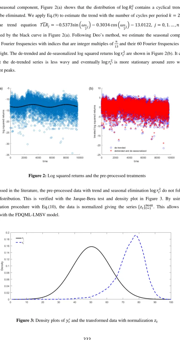
Besides seasonal component, Figure 2(a) shows that the distribution of log𝑅𝑅𝑡𝑡2 contains a cyclical trend that needs to be eliminated. We apply Eq.(9) to estimate the trend with the number of cycles per period 𝑘𝑘= 2. This gives the trend equation 𝑇𝑇𝐿𝐿𝑅𝑅�𝑗𝑗=−0.5373sin�𝜔𝜔𝑛𝑛
2𝑗𝑗� −0.3034 cos�𝜔𝜔𝑛𝑛2𝑗𝑗� −13.0122, 𝑗𝑗= 0, 1. … ,𝑛𝑛 −1 ,
represented by the black curve in Figure 2(a). Following Deo’s method, we estimate the seasonal component based on Fourier frequencies with indices that are integer multiples of 𝑛𝑛
13 and their 60 Fourier frequencies to the
left and right. The de-trended and de-seasonalized log squared returns log𝑟𝑟𝑡𝑡2∗are shown in Figure 2(b). It can be seen that the de-trended series is less wavy and eventually log𝑟𝑟𝑡𝑡2∗is more stationary around zero without significant peaks.
Figure 2: Log squared returns and the pre-processed treatments
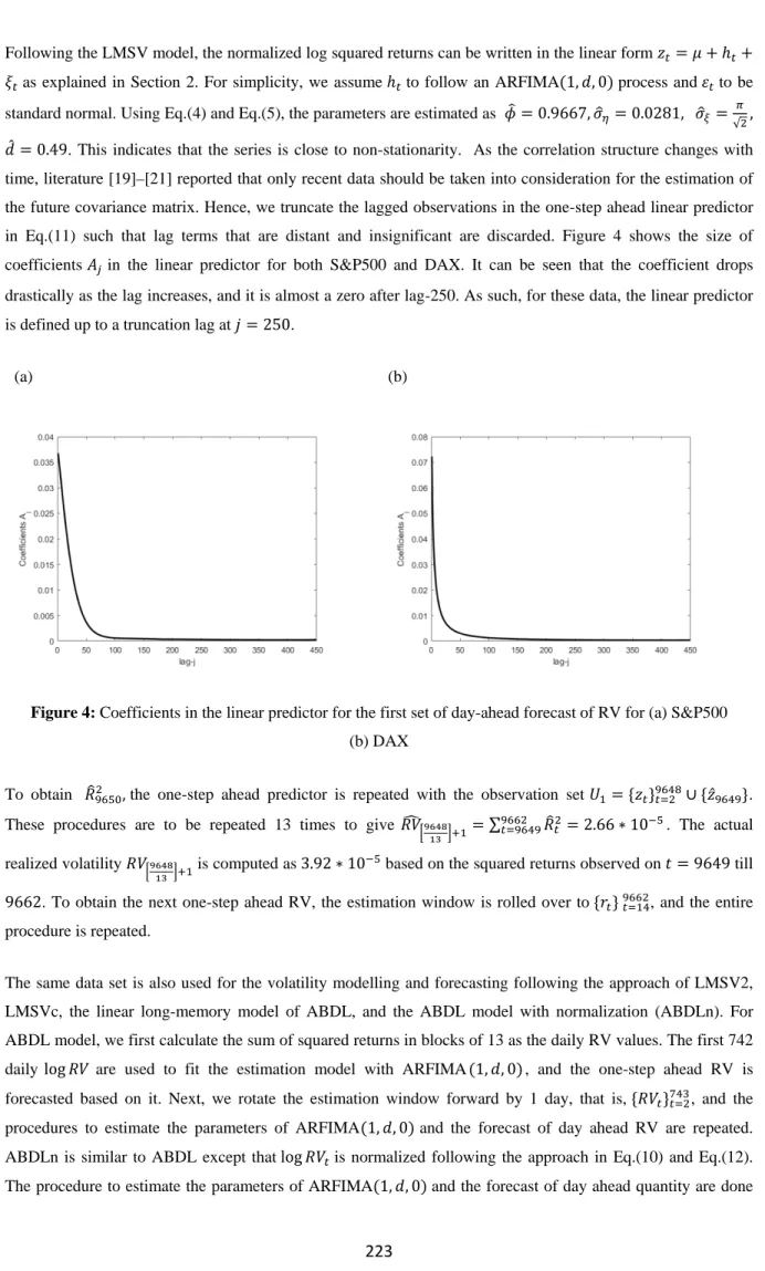
As discussed in the literature, the pre-processed data with trend and seasonal elimination log𝑟𝑟𝑡𝑡2∗do not follow a normal distribution. This is verified with the Jarque-Bera test and density plot in Figure 3. By using the normalization procedure with Eq.(10), the data is normalized giving the series {𝑧𝑧𝑡𝑡}𝑡𝑡=19648. This allows us to proceed with the FDQML-LMSV model.
223
Following the LMSV model, the normalized log squared returns can be written in the linear form 𝑧𝑧𝑡𝑡=𝜇𝜇+ℎ𝑡𝑡+ 𝜉𝜉𝑡𝑡 as explained in Section 2. For simplicity, we assume ℎ𝑡𝑡 to follow an ARFIMA(1,𝑖𝑖, 0) process and 𝜀𝜀𝑡𝑡 to be
standard normal. Using Eq.(4) and Eq.(5), the parameters are estimated as 𝜙𝜙�= 0.9667,𝜎𝜎�𝜂𝜂 = 0.0281, 𝜎𝜎�𝜉𝜉= 𝜋𝜋
√2,
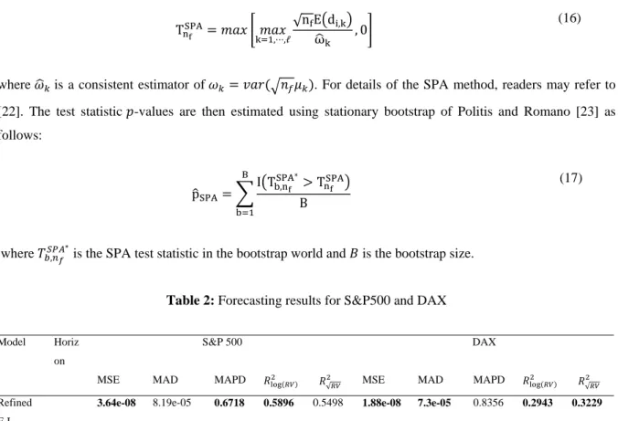
𝑖𝑖̂= 0.49. This indicates that the series is close to non-stationarity. As the correlation structure changes with time, literature [19]–[21] reported that only recent data should be taken into consideration for the estimation of the future covariance matrix. Hence, we truncate the lagged observations in the one-step ahead linear predictor in Eq.(11) such that lag terms that are distant and insignificant are discarded. Figure 4 shows the size of coefficients 𝐴𝐴𝑗𝑗 in the linear predictor for both S&P500 and DAX. It can be seen that the coefficient drops drastically as the lag increases, and it is almost a zero after lag-250. As such, for these data, the linear predictor is defined up to a truncation lag at 𝑗𝑗= 250.
(a) (b)
Figure 4: Coefficients in the linear predictor for the first set of day-ahead forecast of RV for (a) S&P500 (b) DAX
To obtain 𝑅𝑅�96502 , the one-step ahead predictor is repeated with the observation set 𝑈𝑈1= {𝑧𝑧𝑡𝑡}𝑡𝑡=29648∪{𝑧𝑧̂9649}. These procedures are to be repeated 13 times to give 𝑅𝑅𝑅𝑅��9648
13�+1=∑ 𝑅𝑅�𝑡𝑡 2 9662 𝑡𝑡=9649 = 2.66∗10−5. The actual realized volatility 𝑅𝑅𝑅𝑅�9648 13�+1 is computed as 3.92∗10
−5 based on the squared returns observed on 𝑡𝑡= 9649 till
9662. To obtain the next one-step ahead RV, the estimation window is rolled over to {𝑟𝑟𝑡𝑡} 𝑡𝑡=149662, and the entire procedure is repeated.
The same data set is also used for the volatility modelling and forecasting following the approach of LMSV2, LMSVc, the linear long-memory model of ABDL, and the ABDL model with normalization (ABDLn). For ABDL model, we first calculate the sum of squared returns in blocks of 13 as the daily RV values. The first 742 daily log𝑅𝑅𝑅𝑅 are used to fit the estimation model with ARFIMA(1,𝑖𝑖, 0), and the one-step ahead RV is forecasted based on it. Next, we rotate the estimation window forward by 1 day, that is, {𝑅𝑅𝑅𝑅𝑡𝑡}𝑡𝑡=2743, and the procedures to estimate the parameters of ARFIMA(1,𝑖𝑖, 0) and the forecast of day ahead RV are repeated. ABDLn is similar to ABDL except that log𝑅𝑅𝑅𝑅𝑡𝑡 is normalized following the approach in Eq.(10) and Eq.(12). The procedure to estimate the parameters of ARFIMA(1,𝑖𝑖, 0) and the forecast of day ahead quantity are done
224
based on the normalized log𝑅𝑅𝑅𝑅𝑡𝑡. This quantity is then back-transformed by the inverse of Weibull cumulative distribution to give the forecast of day ahead RV following the approach outlined in Section 3.
In the second application, the normalized de-trended and de-seasonalized log squared returns are close to a pure long memory process. The average of the parameter estimates are 𝜙𝜙��= 0.0205,𝜎𝜎��𝜂𝜂= 0.9192,𝜎𝜎��𝜉𝜉= 𝜋𝜋
√2 and
𝑖𝑖̂̅= 0.3894.
To compare the forecast performance of these volatility models, we adopt the measures used in [10], namely (i) the mean squared error (MSE), (ii) the mean absolute deviation (MAD), (iii) the mean absolute percentage deviation (MAPD), (iv) the 𝑅𝑅2 from the regression of log𝑅𝑅𝑅𝑅 on the forecast, log𝑅𝑅𝑅𝑅�, and (v) the 𝑅𝑅2 from the regression of √𝑅𝑅𝑅𝑅 on the forecast, �𝑅𝑅𝑅𝑅�. The results for each combination of forecasting model and horizon for S&P500 and DAX are summarized in Table 2. The best model in the respective performance measure per forecasting horizon is set forth in bold.
It can be seen that the refined FDQML-LMSV model is doing very well if MSE is used as the performance measure. Indeed, it is marked as the best or close to the best model in other performance measures. For S&P500 data set, the proposed model shows the best results in 3 and 4 out of 5 measures for daily and weekly horizons respectively. Although it is not identified as the best model in most of the measures for DAX weekly forecasting horizon, its performances on these measures are rather close to the respective best model.
In line with the findings in [10], we find the ABDL model does an impressive job by just fitting an ARFIMA(1,𝑖𝑖, 0) model to the log squared returns. Interestingly, Table 2 shows that ABDLn does slightly better than ABDL especially when MAPD or 𝑅𝑅2 from the regression of log𝑅𝑅𝑅𝑅 is used.
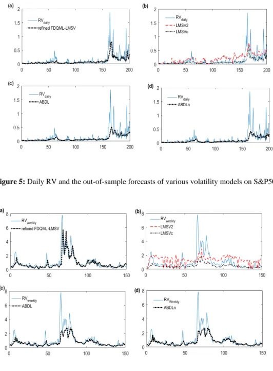
This suggests that the normalization procedure adopted in this study can be a good tool to pre-process data when normality assumption is required. Figures below show the out-of-sample forecast results of various models compared to the daily RV for S&P500 (Figure 5) and weekly RV for DAX (Figure 6).
As a whole, we note that the proposed method is more sensitive to the dynamic of the RV series, and hence producing better forecasts.
To identify the overall best performing model, we additionally run the superior predictive ability (SPA) test ([22], which examines the null hypothesis that the benchmark model is not inferior to any of its competing models. Let’s assume that there are 𝑛𝑛𝑓𝑓 out-of-sample forecasts for the comparison of ℓ+ 1 models. The test statistic is deduced from the loss function differential 𝑖𝑖𝑖𝑖,𝑘𝑘=𝐿𝐿𝑖𝑖,0− 𝐿𝐿𝑖𝑖,𝑘𝑘, 𝑖𝑖= 1,⋯,𝑛𝑛𝑓𝑓, 𝑘𝑘= 1,⋯,ℓ, where 𝐿𝐿𝑖𝑖,0 and 𝐿𝐿𝑖𝑖,𝑘𝑘 are the loss variables of the benchmark model and the competing model-𝑘𝑘 at time 𝑖𝑖 respectively.
Under the assumption of the null hypothesis and that 𝑖𝑖𝑖𝑖,𝑘𝑘 is stationary, we expect that on average, the loss variable of the benchmark model is not bigger than any of the competing model 𝑘𝑘, that is, H0 : max𝑘𝑘=1,⋯,ℓ�𝜇𝜇𝑘𝑘=
225
TnSPAf =𝑚𝑚𝑎𝑎𝑒𝑒 � 𝑚𝑚𝑎𝑎𝑒𝑒k=1,⋯,ℓ√
nfE�di,k�
ω�k , 0�
(16)
where 𝜔𝜔�𝑘𝑘 is a consistent estimator of 𝜔𝜔𝑘𝑘 =𝑐𝑐𝑎𝑎𝑟𝑟(�𝑛𝑛𝑓𝑓𝜇𝜇𝑘𝑘). For details of the SPA method, readers may refer to [22]. The test statistic 𝑝𝑝-values are then estimated using stationary bootstrap of Politis and Romano [23] as follows: p�SPA=� I�TbSPA,nf ∗ > TnSPAf � B B b=1 (17)
where 𝑇𝑇𝑏𝑏𝑆𝑆𝑆𝑆𝐴𝐴,𝑛𝑛𝑓𝑓∗ is the SPA test statistic in the bootstrap world and 𝐵𝐵 is the bootstrap size.
Table 2: Forecasting results for S&P500 and DAX
Model Horiz on
S&P 500 DAX
MSE MAD MAPD 𝑅𝑅log2 (𝑅𝑅𝑅𝑅) 𝑅𝑅
√𝑅𝑅𝑅𝑅
2 MSE MAD MAPD 𝑅𝑅
log(𝑅𝑅𝑅𝑅) 2 𝑅𝑅 √𝑅𝑅𝑅𝑅2 Refined F-L daily
3.64e-08 8.19e-05 0.6718 0.5896 0.5498 1.88e-08 7.3e-05 0.8356 0.2943 0.3229
LMSV2 4.17e-08 1.321e-04 2.18 0.4535 0.4161 2.2e-08 9.15e-05 1.0456 0.1263 0.1624 LMSVc 3.9e-08 8.22e-05 0.7311 0.5789 0.5351 2.6e-08 8.27e-05 0.6253 0.2648 0.2824 ABDL 3.71e-08 8e-05 0.7513 0.5619 0.5563 2.01e-08 7.44e-05 0.8844 0.2604 0.2851 ABDLn 3.85e-08 8.01e-05 0.6942 0.5706 0.5533 1.98e-08 7.41e-05 0.8099 0.2776 0.3066
Refined F-L
weekl y
2.07e-07 2.12e-04 0.4124 0.5815 0.6483 6.55e-07 4.05e-04 0.4019 0.5944 0.6171
LMSV2 6.84e-07 6.21e-04 2.3414 0.3109 0.3702 1.36e-06 8.64e-04 1.44 0.1794 0.1449 LMSVc 2.67e-07 2.34e-04 0.4432 0.5338 0.574 1.24e-06 5.61e-04 0.4206 0.5879 0.5991 ABDL 2.24e-07 2.13e-04 0.4304 0.5827 0.6221 7.37e-07 3.94e-04 0.3365 0.6515 0.6539
ABDLn 2.32e-07 2.15e-04 0.417 0.5907 0.622 7.38e-07 3.97e-04 0.3344 0.6557 0.6518
Note: Refined F-L is the refined FDQML-LMSV model.
In this study, we take the loss variables (𝐿𝐿𝑖𝑖,0 and 𝐿𝐿𝑖𝑖,𝑘𝑘) as the squared error between the forecast and the realized volatility.
The bootstrap 𝑝𝑝-value is generated based on 2000 number of bootstrap resamples. Table 3 shows the results of the SPA-test for the daily and weekly realized volatility forecasts for both S&P500 and DAX indices. It is clear that when the refined FDQML-LMSV model is set as the benchmark, none of the competing model has a smaller squared error, and hence, the null hypothesis is not rejected.
226
Figure 5: Daily RV and the out-of-sample forecasts of various volatility models on S&P500
Figure 6: Weekly RV and the out-of-sample forecasts of various volatility models on DAX
4.1 Economic evaluation of forecasts
As statistical superiority does not necessarily translate to economic benefits, we include the economic evaluation of the forecasts in this study. Value-at-risk (VaR) has been widely used by practitioners and regulators as a measurement of the market risk of financial assets. It is a quantile forecast, of which 𝑅𝑅𝑎𝑎𝑅𝑅𝛼𝛼 is the 𝛼𝛼𝑡𝑡ℎ quantile of the conditional returns. As volatility forecastability is relevant for short time horizons (such as daily trading) and day ahead forecast bears the greatest practical interest [7], [8], we concentrate on the daily VaR forecast that can be written in the equation below.
227
Table 3: SPA-test results for the competing models SPA-test (p-value)
daily weekly
S&P 500 DAX S&P 500 DAX Refined F-L 0 (0.8685) 0 (0.9390) 0 (0.7985) 0 (0.7640) LMSV2 1.0739 (0) 4.1802 (0) 3.8848 (0) 6.4132 (0) LMSVc 1.6144 (0) 2.3150 (0) 1.8094 (0) 1.9612 (0) ABDL 0.2172 (0) 1.2917 (0) 0.5884 (0) 0.7866 (0) ABDLn 1.6994 (0) 1.4366 (0) 0.6825 (0) 0.8682 (0)
Note: The number in the parenthesis is the p-value corresponding to the SPA test statistic.
𝑅𝑅𝑎𝑎𝑅𝑅𝑡𝑡𝛼𝛼𝑑𝑑+1,𝑗𝑗=𝜇𝜇̂𝑡𝑡𝑑𝑑+1,𝑗𝑗+𝜎𝜎�𝑡𝑡𝑑𝑑+1,𝑗𝑗𝐹𝐹𝜚𝜚−1(𝛼𝛼), 𝑡𝑡𝑑𝑑=�
𝑛𝑛
𝑚𝑚�,⋯,𝑛𝑛𝑓𝑓−1 (18) where 𝜇𝜇̂𝑡𝑡𝑑𝑑+1,𝑗𝑗 and 𝜎𝜎�𝑡𝑡𝑑𝑑+1,𝑗𝑗 are the 𝑗𝑗𝑡𝑡ℎ model’s day ahead conditional mean and conditional volatility forecasts respectively, and 𝐹𝐹𝜚𝜚−1 is the inverse cumulative distribution function of the innovations, 𝜚𝜚𝑡𝑡𝑑𝑑= 𝑟𝑟𝑡𝑡𝑑𝑑−𝜇𝜇𝑡𝑡𝑑𝑑
𝜎𝜎𝑡𝑡𝑑𝑑 . From
Table 1, we note that both returns series display similar statistical properties; they are skewed and exhibit fat tails. Here, we estimate the 𝛼𝛼𝑡𝑡ℎ quantile of the 𝜚𝜚𝑡𝑡𝑑𝑑 process using the parametric method based on skewed student distribution, that is, 𝜚𝜚𝑡𝑡𝑑𝑑~𝑖𝑖𝑖𝑖𝑖𝑖𝑐𝑐𝑘𝑘𝑐𝑐𝑡𝑡(0,1,𝜉𝜉,𝜈𝜈), where 𝜉𝜉> 0 is the asymmetry parameter and 𝜈𝜈> 2 is the degree of freedom. The quantity 𝐹𝐹𝜚𝜚−1(𝛼𝛼) is replaced with 𝑐𝑐𝛼𝛼𝑠𝑠𝑘𝑘𝑠𝑠𝑡𝑡,𝜈𝜈,𝜉𝜉 defined in Eq.(19).
228 𝑐𝑐𝛼𝛼𝑠𝑠𝑘𝑘𝑠𝑠𝑡𝑡,𝜈𝜈,𝜉𝜉= ⎩ ⎨ ⎧ (𝜉𝜉−1𝑐𝑐 𝜏𝜏𝑠𝑠𝑡𝑡,𝜈𝜈− 𝑚𝑚)/𝑐𝑐, 𝑤𝑤ℎ𝑒𝑒𝑟𝑟𝑒𝑒 𝜏𝜏=𝛼𝛼2 (1 +𝜉𝜉2), 𝑖𝑖𝑓𝑓𝛼𝛼<1 +1𝜉𝜉2 (−𝜉𝜉𝑐𝑐𝜏𝜏𝑠𝑠𝑡𝑡,𝜈𝜈− 𝑚𝑚)/𝑐𝑐, 𝑤𝑤ℎ𝑒𝑒𝑟𝑟𝑒𝑒 𝜏𝜏=1− 𝛼𝛼2 (1 +𝜉𝜉−2), 𝑖𝑖𝑓𝑓𝛼𝛼 ≥1 +1𝜉𝜉2 (19) where
𝑐𝑐𝜏𝜏𝑠𝑠𝑡𝑡,𝜈𝜈 = the quantile function of the standardized Student-t density function
𝑚𝑚=Γ�𝜐𝜐−12 �√𝜐𝜐−2 √𝜋𝜋Γ�𝜐𝜐2� �𝜉𝜉 − 1 𝜉𝜉� 𝑐𝑐=��𝜉𝜉2+ 1 𝜉𝜉2−1� − 𝑚𝑚2
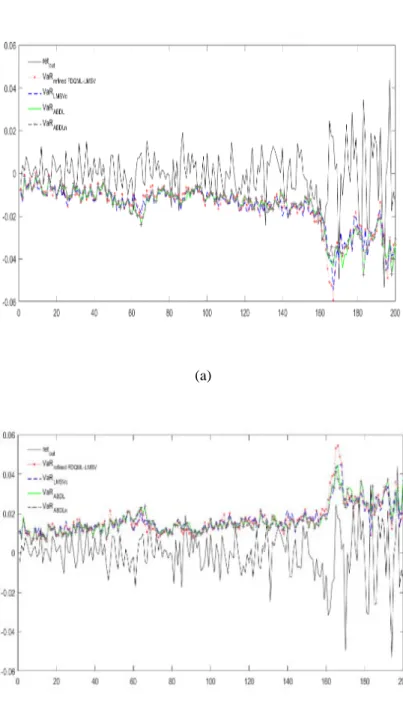
For detailed explanation on the skewed student density function, readers may refer to [7], [24]. To compare the realized volatility models with the economic evaluation, we plug the volatility forecasts into Eq.(18) and compute 5% VaR for both long and short positions. The VaR forecasts compared to the returns series for S&P500 are illustrated in Figure 7. The estimated ex ante VaRs are rather close to each other, and the adequacy of each model needs to be validated. This is done with an evaluation strategy that consists of two steps. First, we examine the statistical accuracy. To verify the null hypothesis that 𝛼𝛼�=𝛼𝛼, we apply the conditional coverage test [25] with the likelihood ratio (LR) given below, of which LR follows an asymptotic 𝜒𝜒2(1) distribution.
𝐿𝐿𝑅𝑅= 2[log(1− 𝛼𝛼�)𝑛𝑛0𝛼𝛼�𝑛𝑛1−log(1− 𝛼𝛼)𝑛𝑛0𝛼𝛼𝑛𝑛1] (20)
where 𝑛𝑛0 is the proportion of failures, 1− 𝛼𝛼�=𝑛𝑛0
𝑛𝑛𝑓𝑓 , and 𝑛𝑛1=𝑛𝑛𝑓𝑓− 𝑛𝑛0.
Next, the models that survive the first step are further evaluated in terms of capital efficiency. We examine this aspect using two popular firm’s loss functions, namely FABL [26] and GK [27]. These functions (for long positions) are given below in Eq.(21) and Eq.(22).
𝐹𝐹𝐴𝐴𝐵𝐵𝐿𝐿𝑡𝑡𝑑𝑑+1,𝑗𝑗=� �𝑅𝑅𝑎𝑎𝑅𝑅𝑡𝑡𝛼𝛼𝑑𝑑+1,𝑗𝑗− 𝑟𝑟𝑡𝑡𝑑𝑑+1� 2 , 𝑖𝑖𝑓𝑓𝑟𝑟𝑡𝑡𝑑𝑑+1<𝑅𝑅𝑎𝑎𝑅𝑅𝑡𝑡𝑑𝑑+1,𝑗𝑗 −𝑐𝑐�𝑟𝑟𝑡𝑡𝑑𝑑+1− 𝑅𝑅𝑎𝑎𝑅𝑅𝑡𝑡𝛼𝛼𝑑𝑑+1,𝑗𝑗�, 𝑖𝑖𝑓𝑓𝑟𝑟𝑡𝑡𝑑𝑑+1≥ 𝑅𝑅𝑎𝑎𝑅𝑅𝑡𝑡𝑑𝑑+1,𝑗𝑗 (21)
where 𝑐𝑐 is the firm’s cost of capital.
𝐺𝐺𝐺𝐺𝑡𝑡𝑑𝑑+1,𝑗𝑗= (𝛼𝛼 − 𝐼𝐼(𝑟𝑟𝑡𝑡𝑑𝑑+1<𝑅𝑅𝑎𝑎𝑅𝑅𝑡𝑡𝛼𝛼𝑑𝑑+1,𝑗𝑗))(𝑟𝑟𝑡𝑡𝑑𝑑+1− 𝑅𝑅𝑎𝑎𝑅𝑅𝑡𝑡𝛼𝛼𝑑𝑑+1,𝑗𝑗) (22)
where 𝐼𝐼(∙) is the indicator function.
The results are further confirmed with the SPA test (see Table 4). Interestingly, it is noted that the normalization procedure in this paper does a good job to improve the accuracy as well as the efficiency in the VaR forecasting. All of the results are tested at 5% significance level, except for S&P500 5% VaR that are examined at 1%
229
significance level due to the marginal adequacy of all of the models. Altough LMSVc is marked as the best model with FABL loss function for the 5% VaR of DAX, this model is also seen as susceptible to inadequacy in other occasions. However, with the proposed improvement, the refined FDQML-LMSV model is robust. It is adequate across all the occasions, and it is identified as the best volatility model that generate efficient VaR in 3 out of 8 efficiency measures. Indeed ABDLn has a higher frequency (4 out of 8); but it leads to inadequate 5% VaR forecasting for S&P500.
(a)
(b)
Figure 7: S&P500 Daily returns and the respective VaR forecasts for (a) 5% long positions (b) 5% short positions
230
Table 4: VaR results for S&P500 and DAX indices
S&P 500 DAX
Statistical accuracy Capital efficiency Statistical accuracy Capital efficiency
LR (p-value) 𝛼𝛼� FABL# (e-07) SPA test (p-value) GK# (e-06) SPA test (p-value) LR (p-value) 𝛼𝛼� FABL# (e-06) 𝑇𝑇𝑆𝑆𝑆𝑆𝐴𝐴 (p-value) GK# (e-06) 𝑇𝑇𝑆𝑆𝑆𝑆𝐴𝐴 (p-value) 5% VaR Refined F-L 5.502 (0.019*) 0.09 7.979 0 (0.5905) 1.302 0 (0.5015) 1.9537 (0.1622) 0.03 1.07 9.4823 (0) 1.22 2.3062 (0) LMSV2 7.0309 (0.008) - - - 0.1088 (0.7416) 0.045 1.07 5.6544 (0) 1.36 2.1208 (0) LMSVc 5.502 (0.019*) 0.09 8.024 0.3075 (0) 1.325 0.34 (0) 0.3968 (0.5287) 0.06 0.835 0 (0.9255) 1.16 0.0265 (0) ABDL 6.8237 (0.009) - - - 1.9537 (0.1622) 0.03 1.07 10.4712 (0) 1.16 0.5816 (0) ABDLn 6.8237 (0.009) - - - 0.4507 (0.502) 0.04 1.03 7.0661 (0) 1.15 0 (0.9465) 95% VaR Refined F-L 0 (1) 0.95 8.75 1.0508 (0) 1.15 1.5771 (0) 1.9537 (0.1622) 0.97 1.09 2.7063 (0) 1.14 0 (0.8705) LMSV2 1.9537 (0.1622) 0.97 12.54 8.2739 (0) 1.39 4.3673 (0) 3.2316 (0.0722) 0.92 1.09 1.1921 (0) 1.36 2.6647 (0) LMSVc 0.1088 (0.7416) 0.955 8.77 1.7075 (0) 1.13 1.1012 (0) 4.3025 (0.0381) - - - - - ABDL 1.0537 (0.3047) 0.965 8.71 4.1125 (0) 1.08 0.2695 (0) 1.0537 (0.3047) 0.965 1.09 4.4767 (0) 1.17 1.3833 (0) ABDLn 0.4507 (0.502) 0.96 8.51 0 (0.928) 1.077 0 (0.9295) 0.4507 (0.502) 0.96 1.05 0 (0.821) 1.16 0.9343 (0) Note:
# FABL and GK are the average values of the firm’s loss functions.
*The bold faced p-values denote rejection of null hypothesis at 0.05 level of significance (except for S&P 500 5%VaR, which are tested at 0.01 level of significance).
5. Conclusion
Modelling high frequency returns using LMSV model has been proposed by [10], but its advantage over the ABDL model is marginal. Focusing on S&P500 and DAX indices, we propose a procedure to eliminate the cyclical trend prior to the de-seasonalization of Deo’s method. Besides, we suggest a parsimonious normalization procedure that makes use of the Gaussian cumulative distribution. To allow a back-transformation, the pre-processed data is fitted with Weibull distribution. The empirical results show that the refined FDQML-LMSV method performs best in MSE across all forecasting horizons and stock indices. Consistent with Deo’s findings, ABDL method is very impressive given that it is a much simpler model. Yet, we note that the model can be further improved with the normalization procedure adopted in this paper. In addition to the statistical superiority, the refined FDQML-LMSV model is also an excellent volatility model to be used with a parametric skewed student distribution in VaR forecasting. The results presented here should be of
231
interest to financial institutions. A risk manager who emphasizes VaR efficiency without disregarding VaR accuracy may focus on the use of refined FDQML-LMSV model as the realized volatility model. However, the proposed model does not consider the financial series that contains a structural break. It would be interesting to see what adjustment to be adapted to the LMSV model to improve the volatility and subsequently the VaR forecasting.
Acknowledgements
We are grateful for the financial support from the Ministry of Higher Education Malaysia (grant: FRGS/1/2014/SG04/UNIM/03/1).
References
[1] T. G. Andersen and T. Bollerslev, “Answering the skeptics: yes, standard volatility models do provide accurate forecasts,” Int. Rev. Econ., vol. 39, pp. 885–905, 1998.
[2] T. G. Andersen, T. Bollerslev, F. X. Diebold, and H. Ebens, “The distribution of realized stock returns volatility,” J. financ. econ., vol. 6, pp. 43–76, 2001.
[3] O. E. Barndorff-Nielsen and N. Shephard, “Econometric analysis of realized volatility and its use in estimating stochastic volatility models,” R. Stat. Soc. Ser. B, vol. 64, pp. 253–280, 2002.
[4] M. Martens, “Measuring and forecasting S&P 500 index-futures volatility using high-frequency data,” J. Futur. Mark., vol. 22, pp. 497–518, 2002.
[5] S. J. Koopman, B. Jungbacker, and E. Hol, “Forecasting daily variability of the S&P100 stock index using historical, realised and implied volatility measurements,” J. Empir. Financ., vol. 12, pp. 445–475, 2005.
[6] M. Martens, D. Dijk, and M. Pooter, “Forecasting S&P 500 volatility: long memory, level shifts, leverage effects, day of the week seasonality and macroeconomic announcements,” Int. J. Forecast., vol. 25, pp. 282–303, 2009.
[7] P. Giot and S. Laurent, “Modeling daily value-at-risk using realized volatility and ARCH type models,” J. Empir. Financ., vol. 11, pp. 379–398, 2004.
[8] D. P. Louzis, S. Xanthopoulos-Sisinis, and A. P. Refenes, “Realized volatility models and alternative Value-at-risk prediction strategies,” Econ. Model., vol. 40, pp. 101–116, 2014.
[9] J. Barunik and T. Krehlik, “Combining high frequency data with non-linear models for forecasting energy market volatility,” Expert Syst. with Appl., vol. 55, pp. 222–242, 2016.
232
volatility model: estimation, prediction and seasonal adjustment,” J. Econom., vol. 131, pp. 29–58, 2006.
[11] F. Corsi, “A simple approximate long-memory model of realized volatility,” J. Financ. Econom., vol. 7, no. 2, p. 174–196., 2009.
[12] T. G. Andersen, T. Bollerslev, F. X. Diebold, and P. Labys, “Modeling and forecasting realized volatility,” Econometrica, vol. 71, no. 2, pp. 579–625, 2003.
[13] B. Cabdelon and L. A. Gil-Alana, “Fractional integration and business cycle features,” Empir. Econ., vol. 29, pp. 1–17, 2004.
[14] G. M. Caporale, J. Cunado, and L. A. Gil-Alana, “Modelling long-run trends and cycles in financial time series data,” J. Time Ser. Anal., vol. 34, pp. 405–421, 2013.
[15] S. Bivona, G. Bonanno, R. Burlon, D. Gurrera, and C. Leone, “Stochastic models for wind speed forecasting,” Energy Convers. Manag., vol. 52, pp. 1157–1165, 2011.
[16] N. Demiris, D. Lunn, and L. D. Sharples, “Survival extrapolation using the poly-Weibull model,” Stat. Methods Med. Res., vol. 24, no. 2, pp. 287–301, 2015.
[17] S. H. Feizjavadian and R. Hashemi, “Analysis of dependent competing risks in the presence of progressive hybrid censoring using Marshall-Olkin bivariate Weibull distribution,” Comput. Stat. Data Anal., vol. 82, pp. 19–34, 2015.
[18] N. Balakrishnan and M. H. Ling, “Best Constant-Stress Accelerated Life-Test Plans With Multiple Stress Factors for One-Shot Device Testing Under a Weibull Distribution,” IEEE Trans. Reliab., vol. 63, no. 4, pp. 944–952, 2014.
[19] F. M. Longin and B. Solnik, “Is the correlation in international equity returns constant,” J. Int. Money Financ., vol. 14, no. 1, pp. 3–26, 1995.
[20] M. C. Munnix, T. Shimada, R. Schafer, F. Leyvraz, T. H. Seligman, T. Guhr, and H. E. Stanley, “Identifying states of a financial market,” Sci. Rep., vol. 2, p. 644, 2012.
[21] T. A. Schmitt, R. Schafer, D. Wied, and T. Guhr, “Spatial dependence in stock returns: local normalization and VaR forecasts,” Empir. Econ., vol. 50, pp. 1091–1109, 2016.
[22] P. R. Hansen, “A test for superior predictive ability,” J. Bus. Econ. Stat., vol. 23, no. 4, pp. 365–380, 2005.
[23] D. N. Politis and J. P. Romano, “The stationary bootstrap,” J. Am. Stat. Assoc., vol. 89, no. 428, pp. 1303–1313, 1994.
233
[24] P. Lambert and S. Laurent, Modelling financial time series using GARCH-type models and a skewed Student density. Mimeo: University of Liege, 2001.
[25] P. Christoffersen, “Evaluating interval forecasts,” Int. Econ. Rev. (Philadelphia)., vol. 39, pp. 841–862, 1998.
[26] P. Abad, S. B. Muela, and C. L. Martin, “The role of the loss function in value-at-risk comparisons,” J. Risk Model Valid., vol. 9, no. 1, pp. 1–19, 2015.
[27] R. Giacomini and I. Komunjer, “Evaluation and combination of conditional quantile forecasts,” J. Bus. Econ. Stat., vol. 23, no. 4, pp. 416–431, 2005.