Measurement based Analysis and Modelling
of UMTS DCH Error Characteristics for
Static Scenarios
Wolfgang Karner, Markus Rupp
Institute of Communications and Radio-Frequency Engineering Vienna University of Technology, Austria
Gusshausstrasse 25/389, A-1040 Vienna, Austria Email:{wkarner, mrupp}@nt.tuwien.ac.at
Abstract— For the evaluation of higher layer
proto-cols, the simulation of cross-layer optimisation methods or the development of new algorithms for multimedia signal processing it is essential to know the exact error characteristics of the underlying channels. In this paper we show the analysis of the error characteristics of the UMTS DL (Down Link) DCH (Dedicated Channel) with 384kbit/s especially for static scenarios. The analysis is based on measurements in live UMTS networks in Vienna, Austria and the results are compared to the ob-tained statistics of measurements in a reference network where the transmission of data was performed without interference from other cells, multipath propagation or fading effects. Following the obtained statistics we develop a two-state model which is capable of describ-ing the measured statistics properly. Furthermore, we analyse the correlation properties of the channel and we show a two-layer model for an improved representation of the statistical dependencies between the errors of the UMTS DL DCH.
I. INTRODUCTION
In digital wireless transmission systems the link errors have a great impact on the performance of the higher layer protocols [1] due to the statistical dependencies between the errors. In contrast to wired links, in wireless systems the errors are often grouped together in bursts because of the high variability of the radio link. That influences the functionality of the higher layer protocols more severely than the equally distributed transmission errors of wired sys-tems. Thus, it is all-important to be aware of the error characteristics of the used channel when developing new algorithms for multimedia signal processing or optimising the protocol stack for wireless transmission systems.
Due to the high flexibility - especially of the 3G mobile communication networks - lots of different and new applications and protocols, as well as multimedia signal processing algorithms or cross-layer optimisa-tion methods like in [2] are currently developed for UMTS. The development procedure highly depends on the properties of the underlying system. Therefore, it is very important to analyse the error characteristics of the UMTS DCH (Dedicated Channel) beforehand as it is used by most of the services.
In several publications the behaviour of the UMTS DCH has been investigated by link level or physical layer simulations [3]. Our approach in this paper is to provide an analysis of the error characteristics of the UMTS DCH based on measurements in live UMTS networks in Vienna, Austria. We are particularly fo-cussing on the error characteristics of the UMTS DCH in the DL (Down Link) with a throughput of 384kbit/s for static scenarios. This is the typical configuration when using a UMTS PCMCIA datacard or a mobile phone as a modem in connection with a notebook.
For evaluation of the performance of protocols or algorithms, exhaustive simulations have to be per-formed where the lower layers are represented e.g. by stochastic models. In this paper we develop models, following the measured statistics, which are capable of describing the error characteristics of the UMTS DL DCH for 384kbit/s properly for the static case.
In order to observe the influence of the propagation effects like multipath propagation or fading1 on the error characteristics, we are comparing the measure-ment results of the live network with the results of the reference network. In the reference network the measurements can be performed with the mobile enclosed within a shielding box which is directly connected to the antenna connector of the Node B.
This document is organised as follows. In Sec-tion II the measurement setup will be explained and the utilised parameters for traffic and system will be presented. Section III shows the analysis of the error characteristics of the UMTS DL DCH. First an analysis of the gap- and burstlengths2will be presented and then we show the results of the analysis of the correlation properties. In Section IV one possible way of modelling the error characteristics via a two-state model is presented. Furthermore, a two-layer model as an enhancement for the two-state model is shown, which is capable of describing the correlation properties more accurately. Finally, in Section V a summary and conclusions will be given.
1Fading is present in a small amount also in static scenarios. 2Gaplength/burstlength is the number of subsequently received
error free/erroneous transport blocks.
8th International Symposium on DSP and Communication Systems, DSPCS'2005" & "4th Workshop on the Internet, Telecommunications and Signal Processing, WITSP'2005", Noosa Heads (Sunshine Coast, Australia), 19-21 December 2005
II. MEASUREMENTSETUP
A. General Setup
The measurements results for this work are based on measurements in three live UMTS networks of three different operators in the city center of Vi-enna, Austria. Measurements in the three networks have shown great similarity for the static case [4]. Therefore, we are presenting in this document the measurements out of only one operator’s live network, but at three different locations. Additionally, we show the measurements performed in the reference network (a separate network for acceptance testing) of the same operator, where corresponding parameters can be adjusted. USB PC RNC SGSN GGSN Node B TU-Vienna Internet Uu Iub Iu/PS Gn Gi
UDP const. kbit/s
TEMS Investigation WCDMA Iub Iu/PS RNC Node B PC SGSN GGSN TU-Vienna Internet USB
UDP const. kbit/s TEMS Investigation
WCDMA
Gn Gi
shielding box
Fig. 1. Measurement setup, live network/reference network. For the measurements a UDP data stream with a bit rate of 360kbit/s (372kbit/s incl. UDP/IP overhead) in DL was used. The data was sent from a PC located at the Institute of Communications and Radio Frequency Engineering at the Vienna University of Technology to a notebook using a UMTS terminal as a modem. As depicted in Fig. 1 (upper part), during the measurements in the live network the UDP data stream goes from the PC over University LAN (ethernet), internet, UMTS core network and over the UMTS air interface (with a 384kbit/s radio access bearer assigned during the measurements in DL) to a UMTS mobile which is connected via USB (Universal Serial Bus) to the notebook. In order to represent a static scenario the mobile terminal was lying on a table in an office or living room with only few movements of objects or persons around the mobile during the measurements.
In case of the measurements in the reference net-work the signal is routed via coaxial cable to a shielding box directly from the antenna connector of the Node B as can be seen in Fig. 1 (lower part). In that shielding box the UMTS terminal is enclosed in order to avoid inter-cell interference, multipath propagation effects and fading.
The statistics of CPICH Ec/I0 (Common Pilot
Channel chip energy to noise and interference ratio)
location 1 0 2000 4000 6000 8000 10000 12000 -10 -9 -8 -7 -6 -5 -4 -3 -2 -1 0 CPICH Ec/I0 [dB] h is to g ra m location 2 0 10000 20000 30000 40000 50000 60000 -10 -9 -8 -7 -6 -5 -4 -3 -2 -1 0 CPICH Ec/I0 [dB] h is to g ra m location 3 0 2000 4000 6000 8000 10000 12000 14000 16000 -10-9 -8 -7 -6 -5 -4 -3 -2 -1 0 CPICH Ec/I0 [dB] h is to g ra m reference network 0 5000 10000 15000 20000 25000 30000 35000 -10 -9 -8 -7 -6 -5 -4 -3 -2 -1 0 CPICH Ec/I0 [dB] h is to g ra m
Fig. 2. CPICHEc/I0at diff. locations in the live network and in
the reference network.
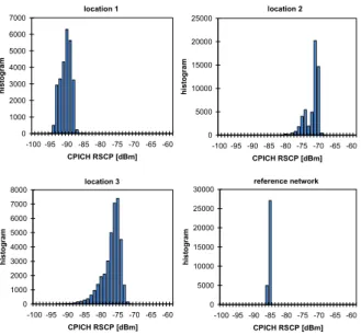
location 1 0 1000 2000 3000 4000 5000 6000 7000 -100 -95 -90-85-80 -75-70-65 -60 CPICH RSCP [dBm] h is to g ra m location 2 0 5000 10000 15000 20000 25000 -100 -95-90-85-80-75-70 -65-60 CPICH RSCP [dBm] h is to g ra m location 3 0 1000 2000 3000 4000 5000 6000 7000 8000 -100 -95-90 -85-80-75-70-65 -60 CPICH RSCP [dBm] h is to g ra m reference network 0 5000 10000 15000 20000 25000 30000 -100 -95 -90 -85 -80 -75 -70 -65 -60 CPICH RSCP [dBm] h is to g ra m
Fig. 3. CPICHRSCP at diff. locations in the live network and in the reference network.
and CPICH RSCP (CPICH Received Signal Code
Power) during the measurements are shown in Fig. 2 and Fig. 3 respectively. There can be observed that the values for CPICHEc/I0 and CPICHRSCP are
in the same regions in the measurements of live-and reference network, but there is no fading in the reference network. There was additional traffic during the measurements in the live network, but the used cells were not heavy loaded and there was a 384kbit/s bearer assigned for the measurement data stream in DL for the whole measurement period. Furthermore, measurements in heavy loaded cells have shown that the cell load has no impact on the DCH error charac-teristics.
A WCDMA TEMS mobile3 (Motorola A835) was used as terminal. On the notebook the measurements of the mobile have been captured by ‘TEMS Inves-tigation WCDMA 2.4’ software also by Ericsson. By parsing the export files of this software tool, the BLER (Block Error Ratio), burstlengths, gaplengths and other parameters have been analysed as explained further on in this paper.
Of course we are aware of the disadvantage of measuring with one type of mobile terminal only. However, the Motorola A835 was the only TEMS mo-bile station available to us and capable of presenting the CRC (Cyclic Redundancy Check) information of the received transport blocks. The error characteristics of the Motorola A835 are assumed to be comparable to the error characteristics of other mobiles because similar results have been observed when comparing the measured statistics of the BLER (Block Error Ra-tio) of the Motorola A835 with the statistics collected with Sony Ericsson Z1010 mobile terminals.
B. Relevant UTRAN Parameters
In the considered UMTS networks in Vienna, the relevant system parameters are as follows.
As TrCH (Transport Channel) in the DL a DCH (Dedicated CHannel) and RLC AM (Acknowledged Mode) has been used. In addition, turbo coding and a transport block size of 336 bits has been selected. For the 384kbit/s bearer the SF (Spreading Factor) was 8 and the TTI (Transmission Timing Interval) was 10ms with 12 transport blocks per TTI.
Another very important parameter of the UTRAN for evaluating the error characteristics of the DCH is the BLER quality target value for the outer loop TPC (Transmit Power Control) which was set to 1% in the networks used for the measurements. As a consequence the closed outer loop TPC tries to adjust the SIR (Signal to Interference Ratio) target for the closed inner loop (fast) TPC in a way that the required BLER quality (1% in our case) is satisfied.
III. ANALYSIS OFDL DCH ERROR CHARACTERISTICS
A. Analysis of gaplength and burstlength
In [4] we have shown a method for analysing the error characteristics of the UMTS DCH based on TTIs, which means we have been looking at subsequent TTIs and if they contain an erroneous transport block or not. The reason for using that method of analysing the DCH was that in scenarios with mobility the probability is 80-85% to receive all 12 transport blocks erroneous within one TTI - considering only erroneous TTIs.
In static scenarios, the probability of receiving all transport blocks (trbks) of a TTI in error (12 trbks in 3A modified Motorola A835 for TEMS data logging, offered by
Ericsson [5]. Modifications are only done in order to provide internal measurements via the interface.
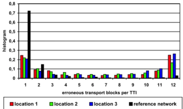
0 0,1 0,2 0,3 0,4 0,5 0,6 0,7 0,8 1 2 3 4 5 6 7 8 9 10 11 12
erroneous transport blocks per TTI
h is to g ra m
location 1 location 2 location 3 reference network
Fig. 4. Measured number of erroneous transport blocks per TTI.
case of the 384kbit/s bearer), is only around 20% as can be seen in Fig. 4. The probability of having only one erroneous transport block within one erroneous TTI is as well around 20% in the measurements of the live network and even more than 70% in the reference network.
Due to that fact, the analysis of the error character-istics of the UMTS DCH for the static case should be based on transport blocks rather than on TTIs.
trbk
trbk
…erroneous transport block
gaplength burstlength
trbk trbk trbk trbk trbk trbk trbk trbk trbk trbk trbk trbk trbk
…error free transport block
trbk
Fig. 5. Analysis of DCH error characteristics based on transport blocks.
An analysis method for the error characteristics of the DCH by the measured data is depicted in Fig. 5. The method builds on the observation of the state of the transport blocks. We are looking particularly for the number of subsequent error free trbks what we call the gaplength while the number of subsequent erroneous trbks is called burstlength. The definition of an error burst is according to [6] where a burst is a group of bits in which two successive erroneous bits are always separated by less than a given number L of correct bits. In our case L is equal to zero.
The statistics of gaplengths and burstlengths ob-tained from measurements in the static case - at different locations in the live network and in the reference network - is presented in Figs. 6 and 7.
As can be seen in Fig. 6, there are two areas where the gaplengths occur with a higher probability. One is the part of long gaps with more than 1000 subsequent error free trbks and the other part is with gaps≤12. Our assumption for the reason of the long gaps is the period of the OLPC (Outer Loop Power Control) when it is built like proposed in [7]. In the ideal case (without any disturbance) the period of the OLPC would be 100 for reaching a BLER target of 1% and the gaplength would be 99. Due to the burstiness of the errors the period (and therefore the gaplengths)
100 101 102 103 104 0 0.1 0.2 0.3 0.4 0.5 0.6 0.7 0.8 0.9 1
gaplength (number of transport blocks)
empirical CDF
static, location 3 static, location 2 static, location 1 static, reference network
Fig. 6. Measured gaplength in number of trbks, diff. locations. become>1000. The short gaps could be attributed to
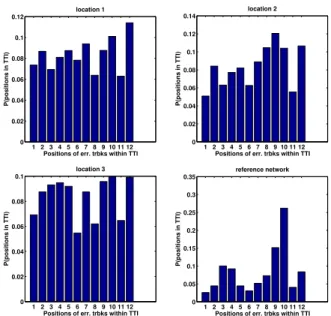
the multipath propagation and fading because they are less probable in the reference network. Another reason for having gaps≤12could be due to effects of turbo coding. As shown in [8], the turbo coder produces bit errors which are equally distributed across the coding block (TTI). We can see in Fig. 8 that the erroneous transport blocks have also almost equally distributed positions within the TTI in the live network. Fig. 9 illustrates that short gaps can result in such a case.
0 5 10 15 20 25 0 0.1 0.2 0.3 0.4 0.5 0.6 0.7 0.8 0.9 1
burstlength (number of transport blocks)
empirical CDF
static, location 1 static, location 2 static, location 3 static, reference network
Fig. 7. Measured burstlength in number of trbks, diff. locations. Fig. 7 shows the measured burstlengths (number of subsequent erroneous transport blocks) depicted as empirical cdf. It can be observed that the bursts have a length between one and 25 and the probability of burstlength one is almost 90% in the reference network and around 50% in the live network. At burstlengths of 12 and 24, larger steps occur in the empirical cdf which is due to the fact that also in the static case the probability of receiving all (12) transport blocks in error within one TTI is quite high.
B. Analysis of DL DCH Error Correlation Properties
From the statistics of gap- and burstlengths (Figs. 6, 7) we can already come to the conclusion that there is correlation between the error states of subsequent transport blocks due to the burstiness of the errors. As can be observed, the errors are grouped together in bursts of lengths≤24trbks, separated by
gaps with>1000trbks. 1 2 3 4 5 6 7 8 9 10 11 12 0 0.02 0.04 0.06 0.08 0.1 0.12
Positions of err. trbks within TTI
P(positions in TTI) location 1 1 2 3 4 5 6 7 8 9 10 11 12 0 0.02 0.04 0.06 0.08 0.1 0.12 0.14
Positions of err. trbks within TTI
P(positions in TTI) location 2 1 2 3 4 5 6 7 8 9 10 11 12 0 0.02 0.04 0.06 0.08 0.1
Positions of err. trbks within TTI
P(positions in TTI) location 3 1 2 3 4 5 6 7 8 9 10 11 12 0 0.05 0.1 0.15 0.2 0.25 0.3 0.35
Positions of err. trbks within TTI
P(positions in TTI)
reference network
Fig. 8. Probability of positions of erroneous transport blocks within TTI.
TTI, 10ms trbk
Fig. 9. Schematic illustration of erroneous transport blocks within one TTI.
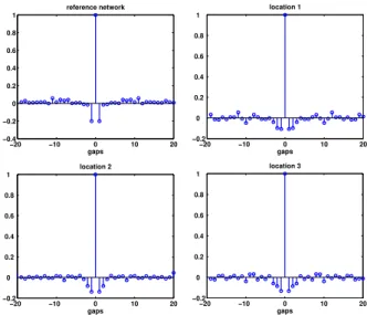
Another very important property is the statistical de-pendency between subsequent gaps, subsequent bursts and between gaps and bursts. In Fig. 10 the schematic illustration of uncorrelated (memoryless) and corre-lated gaps and bursts is shown. When looking at the autocorrelation function of subsequent gaps in Fig. 11, one can observe the present correlation between at least the nearest neighbours of subsequent gaps. To analyse the statistical independency between two suc-cessive gaps, the simple and conditional probabilities (conditioned on the length of the previous gap) of
burstlength gaplength burstlength: iid gaplength: iid uncorrelated (memoryless): iid iid …erroneous trbk …error free trbk correlated: stat. dependency stat. dependency stat. dependency stat. dependency
having a gaplength of≤12 and>12§, are shown in
Fig. 12. As the simple and conditional probabilities are different, there is no statistical independence between subsequent gaplengths. Similar results can be shown for subsequent burstlengths and between a gap and the following burst. In order to capture these statistical dependencies appropriately we propose the two-layer model presented in Section IV B.
−20 −10 0 10 20 −0.4 −0.2 0 0.2 0.4 0.6 0.8 1 gaps reference network −20 −10 0 10 20 −0.2 0 0.2 0.4 0.6 0.8 1 gaps location 1 −20 −10 0 10 20 −0.2 0 0.2 0.4 0.6 0.8 1 gaps location 2 −20 −10 0 10 20 −0.2 0 0.2 0.4 0.6 0.8 1 gaps location 3
Fig. 11. Autocorrelation functions of gaplengths.
1 2 0 0.1 0.2 0.3 0.4 0.5 0.6 0.7 location 1 1 2 0 0.1 0.2 0.3 0.4 0.5 0.6 0.7 location 2 1: P(gap<=12), 2: P(gap>12)
1: P(gap(n)<=12 | gap(n−1)<=12), 2: P(gap(n)>12 | gap(n−1)<=12) 1: P(gap(n)<=12 | gap(n−1)>12), 2: P(gap(n)>12 | gap(n−1)>12)
1 2 0 0.1 0.2 0.3 0.4 0.5 0.6 0.7 location 3 1 2 0 0.1 0.2 0.3 0.4 0.5 0.6 0.7 0.8 reference network
Fig. 12. Conditional probabilities of subsequent gaplengths. IV. MODELLING OFDL DCH ERROR
CHARACTERISTICS
In literature, many different ways of modelling the error sequences of digital mobile channels have been
§The probabilities of ≤
12and > 12 have been chosen for
that analysis in view of the following modelling of the error characteristics in Section IV.
proposed beginning with [9], [10] and [11] by the use of Markov chains, hidden Markov models [12] [13] or several other methods. In order to describe the desired statistics of gaplengths and burstlengths ideally, anN -state Markov model with largeN would be necessary. As our intention is to keep the complexity of the model as small as possible our first approach is a two-state model (renewal process), which only has a few easy determinable parameters and is suitable for modeling the error characteristics of the UMTS DCH with uncorrelated gaps and burst. This modelling approach is explained in the following subsection.
A. Two-state Model
The goal in modelling the error characteristics of the UMTS DCH in this subsection is to generate a sequence of transport blocks with the correct statistics of gaplengths and burstlengths. As already mentioned in Section III (Fig.6), there are two main areas with high probability of gaplengths - long gaps with more than 1000 subsequent error free trbks and short gaps with≤12trbks. We are using the same partitioning of
gaplengths for modelling of the statistics. As shown in Fig. 13 for location 1 in the live network, the statistics of small gaplengths can properly be modelled via a Weibull distribution with scale parameter as 1.2 and shape parameter be 0.7. 0 2 4 6 8 10 12 0 0.1 0.2 0.3 0.4 0.5 0.6 0.7 0.8 0.9 1
gaplength (number of transport blocks)
empirical CDF
measurement, location 1 simulation, Weibull (1.2,0.7)
Fig. 13. Measurement vs. simulation of gaplengths≤12trbks,
location 1. 0 2000 4000 6000 8000 10000 0 0.1 0.2 0.3 0.4 0.5 0.6 0.7 0.8 0.9 1
gaplength (number of transport blocks)
empirical CDF
measurement, location 1 simulation, Weibull (3350, 2.0167)
Fig. 14. Measurement vs. simulation of gaplengths>12trbks,
The two-parameter Weibull CDF is given by F(x|a, b) = Z x 0 ba−btb−1e−(ta) b dt (1)
where a and b are scale and shape parameters,
re-spectively. A Weibull distribution also meets the sta-tistics of the gaps with > 12 trbks (Fig. 14) with
a = 3350 and b = 2.0167, again shown for the
measurement at location 1 in the live network. The combination of these two Weibull distributions now is capable of describing the total statistics of measured gaplengths adequately (see Fig. 15). The comparison between the measured and simulated statistics of the burstlengths at location 1 in the live network is shown in Fig. 16, where again a Weibull distribution is used for modelling, supplemented by additional steps at the burstlengths of 12 and 24.
The reason for using a Weibull distribution in mod-elling gap and burst statistics is the high flexibility of the two-parameter Weibull distribution [14]. By proper adjustment of the shape parameter, exponential-, Rayleigh-exponential-, normal- and even other distributions can be met or approximated. 100 101 102 103 104 0 0.1 0.2 0.3 0.4 0.5 0.6 0.7 0.8 0.9 1
gaplength (number of transport blocks)
empirical CDF
measurement, location 1 simulation, two−part Weibull
Fig. 15. Measurement vs. simulation of gaplengths (two-part Weibull distribution), location 1.
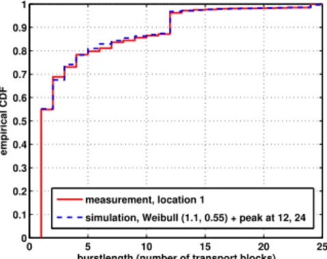
0 5 10 15 20 25 0 0.1 0.2 0.3 0.4 0.5 0.6 0.7 0.8 0.9 1
burstlength (number of transport blocks)
empirical CDF
measurement, location 1
simulation, Weibull (1.1, 0.55) + peak at 12, 24
Fig. 16. Measurement vs. simulation of burstlengths, location 1. Following the explained method of describing ad-equate statistics for gap- and burstlengths we arrive at a two-state model as shown in Fig. 17, where in one state correct transport blocks and in the other state erroneous transport blocks are generated. In the correct state, the number of subsequent error free transport
blocks (gaplength) is calculated via a two-part Weibull distributed random number and the number of sub-sequent erroneous transport blocks (burstlength) in the error state is calculated via a simple Weibull distributed random number but with additional peaks at burstlengths of 12 and 24. After each calculation of either burst- or gaplength, the state is changed. Therefore, for modelling the error characteristics of the UMTS DCH in this way, a total number of nine parameters are required. These are: four parameters for the two Weibull distributions and one parameter for the separation between the distributions in the correct state. Additionally, two parameters for the Weibull distribution and two parameters for determination of the peaks at 12 and 24 in the erroneous state.
state: trbks correct gaplength = two-part Weibull
distributedrandom number
state: trbks in error burstlength =Weibull distributed
random number + peaks at 12,24
Fig. 17. Two-state model.
B. Two-Layer Model for modelling Correlation Prop-erties
The two-state model mentioned in the previous subsection is a renewable process, meaning there is no dependency between subsequent gaps, subsequent bursts or neither between a gap and the following burst (see the schematic illustration in Fig. 10). On the other hand - as shown in Section III B - there is statistical dependency between subsequent gaps, bursts and also between a gap and the following burst. Therefore we propose the following two-layer model (kind of hidden Markov model) where correlation between gaps and bursts is introduced via the upper layer two-state Markov chain (Fig. 18).
pss psl pll pls state: trbks correct state: trbks in error state: trbks correct state: trbks in error short state gaplength <= 12 long state gaplength > 12
Fig. 18. Two-layer two-state Markov model.
The model has one ’short state’ (gaps with ≤ 12
trbks) and one ’long state’ (gaps with > 12 trbks) and the corresponding transition probabilities are the conditional probabilities out of Fig. 12. After entering a certain state, first the gaplength is calculated via a Weibull distributed random number for either the small or the large gaplengths according to the separation in Section III and depending on the current upper layer state. Then, while staying in the same state of the upper layer Markov chain, a burst is calculated with different probabilities of either creating a Weibull distributed burstlength or a peak at 12 or 24, again depending on the actual upper layer state. After that
the state of the upper layer Markov chain is changed and the procedure begins again with calculating the gaplength.
Thus, via the upper layer Markov chain, the model introduces correlation between subsequent gaps and also between a gap and the following burst by us-ing 11 parameters. Two parameters are necessary for determination of the transition probabilities of the upper layer Markov chain. Another two parameters are used for the Weibull distributions of each of the correct states and only two parameters more for the Weibull distributions of both erroneous states as the Weibull distributions are the same for the erroneous states of both upper layer states. What depends on the current state of the upper layer Markov chain in case of the erroneous states is the probability of generating Weibull distributed burstlenghts or having a burst with lengths 12 or 24. For these probabilities and the separation between a burstlength of 12 and 24 another three parameters are needed.
We can see the improvements in modelling the error characteristics by using this correlated model in the following subsection.
C. Simulation Results
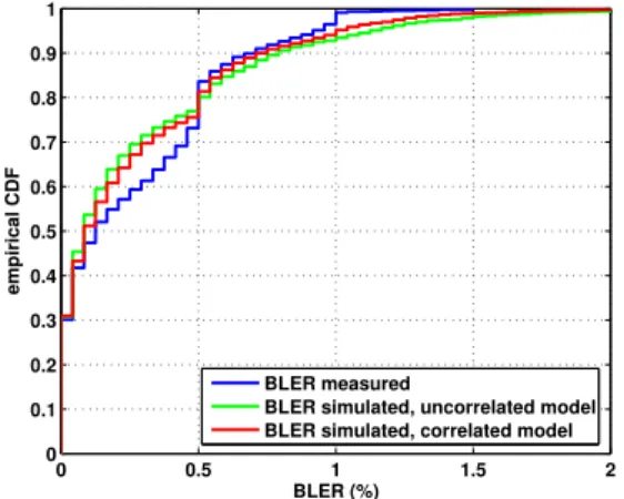
In this subsection we are comparing the simulated results of the two presented models with the mea-sured statistics. In Fig. 19 the empirical CDF of the error weight probability P(m,n), the probability of exactly m errors occurring in a block of n, is shown which we call the Block Error Ratio (BLER) with n equal to 2400 trbks. We can see that the uncorrelated two-state Model is able to describe the measured statistics quite well although it does not meet the correct correlation properties of the channel. This can be seen in the absence of the bigger steps at 0.5% and 1%. The correlated model is bringing an observable enhancement to the problem by using two more parameters. Of course, the two-layer model only catches a part of the correlation characteristics of the channel. Therefore, only small improvements compared to the uncorrelated model can be achieved.
0 0.5 1 1.5 2 0 0.1 0.2 0.3 0.4 0.5 0.6 0.7 0.8 0.9 1 BLER (%) empirical CDF BLER measured
BLER simulated, uncorrelated model BLER simulated, correlated model
Fig. 19. Comparison of BLER measurements and simulation results of the models, location 1.
V. SUMMARY ANDCONCLUSIONS
We have shown the analysis of the error charac-teristics of the UMTS DCH (Dedicated Channel) in DL (Down Link) for static scenarios, based on mea-surements in live UMTS networks in Vienna, Austria. We present statistics of gap- and burstlengths which are furthermore compared to the statistics obtained in a reference network, where transmission without multipath propagation or fading is possible. It is shown that these statistics can all be perfectly matched by Weibull distributions because of the great flexibility the two-parameter Weibull distribution offers in its shape parameter. Following the measured statistics we have developed a two-state model describing a renew-able process which is caprenew-able of meeting the statistics of gap- and burstlengths properly. Additionally we analyse the correlation properties between subsequent gaps and bursts and it is shown that there is no statistical independence. Thus, we further propose a two-layer model (kind of hidden Markov model) as an enhancement to the simple two-state model.
ACKNOWLEDGEMENTS
We thank mobilkom austria AG&CoKG for tech-nical and financial support of this work. The views expressed in this paper are those of the authors and do not necessarily reflect the views within mobilkom austria AG&CoKG.
REFERENCES
[1] M. Zorzi, R.R. Rao, “Perspectives on the Impact of Error Statistics on Protocols for Wireless Networks”, IEEE Personal Communications, Vol. 6, pp. 32–40, Oct. 1999.
[2] O. Nemethova, W. Karner, A. Al-Moghrabi, M. Rupp, “Cross-Layer Error Detection for H.264 Video over UMTS,” inProc. of Wireless Personal Multimedia Communications 2005 (WPMC 2005), Aalborg, Denmark, Sept. 2005.
[3] J.J. Olmos, S.Ruiz, “Transport Block Error Rates for UTRA-FDD Downlink with transmission Diversity and Turbo coding,” inProc. IEEE 13th PIMRC 2002, vol.1, pp 31-35, Sept. 2002. [4] W. Karner, P. Svoboda, M. Rupp, “A UMTS DL DCH Error Model Based on Measurements in Live Networks,” in Proc. of 12th International Conference on Telecommunications 2005 (ICT 2005), Capetown, South Africa, May 2005.
[5] http://www.ericsson.com/products/hp/TEMS Products pa.shtml [6] ITU-T Rec. M.60, 3008; ITU-T Rec. Q.9, 0222.
[7] H. Holma and A. Toskala,WCDMA for UMTS, Radio Access For Third Generation Mobile Communications, Third Edition,
John Wiley & Sons, Ltd., 2004.
[8] F. Navratil, “Fehlerkorrektur im physical Layer des UMTS,” Master’s thesis, Institute of Communications and Radio-Frequency Engineering, Vienna University of Technology, Aus-tria, Nov. 2001.
[9] E.N. Gilbert, “Capacity of a burst-noise channel,”Bell Systems Technical Journal, vol. 39, pp. 1253–1265, Sept. 1960. [10] E.O. Elliot, “Estimates of error rates for codes on burst-noise
channels,”Bell Systems Technical Journal, vol. 42, pp. 1977– 1997, Sept. 1963.
[11] B.D. Fritchman, “A Binary Channel Characterization Using Partitioned Markov Chains,” IEEE Trans. Information Theory, vol. 13, no. 2, pp. 221–227, Apr. 1967.
[12] W. Turin,Digital Transmission Systems: Performance Analysis and modelling. New York: McGraw-Hill, 1999.
[13] L.R. Rabiner, B.H. Juang, “An Introduction to Hidden Markov Models,” IEEE ASSP Magazine, Vol. 3, pp. 4–16, Jan. 1986. [14] http://www.weibull.com/lifedatawebcontents.htm#Introduction