UCLA
UCLA Electronic Theses and Dissertations
TitleFundamental Results on Asynchronous Parallel Optimization Algorithms Permalink
https://escholarship.org/uc/item/5qf644g6 Author
Hannah, Robert Rafaeil Publication Date 2019
Peer reviewed|Thesis/dissertation
UNIVERSITY OF CALIFORNIA Los Angeles
Fundamental Results on Asynchronous Parallel
Optimization Algorithms
A dissertation submitted in partial satisfaction of the requirements for the degree Doctor of Philosophy in Mathematics
by
c
Copyright by Robert Rafaeil Hannah
ABSTRACT OF THE DISSERTATION
Fundamental Results on Asynchronous Parallel
Optimization Algorithms
by
Robert Rafaeil Hannah
Doctor of Philosophy in Mathematics University of California, Los Angeles, 2019
Professor Wotao Yin, Chair
In this thesis, we present a body of work on the performance and convergence properties of asynchronous-parallel algorithms completed over the course of my doctorate degree (Hannah, Feng, and Wotao Yin 2018; Hannah and Wotao Yin 2017b; T. Sun, Hannah, and Wotao Yin 2017; Hannah and Wotao Yin 2017a). Asynchronous algorithms eliminate the costly synchronization penalty of traditional synchronous-parallel algorithms. They do this by having computing nodes utilize the most recently available information to compute updates. However, it’s not immediately clear whether the trade-off of eliminating synchronization penalty at the cost of using outdated information is favorable.
We first give a comprehensive theoretical justification of the performance advantages of asynchronous algorithms, which we summarize as "Faster Iterations, Same Quality" (Hannah and Wotao Yin 2017a). Under a well-justified model, we show that asynchronous algorithms complete "Faster Iterations". Using renewal theory, we demonstrate how network delays, heterogeneous sub-problem difficulty and computing power greatly hinder synchronous algorithms, but have no impact on their asynchronous counterparts. We next prove the first exact convergence rate results for a variety of synchronous algorithms including synchronous ARock and synchronous randomized block coordinate descent (sync-RBCD). This allows us
Finally we show that a variety of asynchronous algorithms have a convergence rate that essentially matches the previously derived exact rates for synchronous counterparts so long as the delays are not too large. Hence asynchronous algorithms complete faster iteration that are of the "Same Quality" as synchronous algorithms. Therefore we conclude that a wide variety of asynchronous algorithms will always outcompete their synchronous counterparts if the delays are not too large, and especially at scale.
Next we present the first asynchonous Nesterov-accelerated algorithm that attains a speedup: A2BCD (Hannah, Feng, and Wotao Yin 2018). We first prove that A2BCD attains
NU_ACDM’s complexity to highest order. NU_ACDM is a state-of-the-art accelerated coordinate descent algorithm (Allen-Zhu, Qu, et al. 2016). Then we show that both A2BCD andNU_ACDM
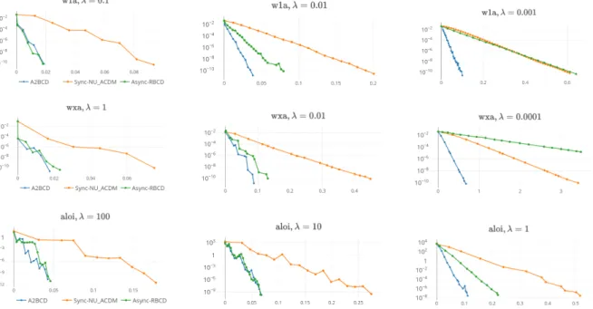
both have optimal complexity. Hence because A2BCD has faster iterations, and optimal complexity, it should be the fastest coordinate descent algorithm. We verify this with numerical experiments comparing A2BCD with NU_ACDM. We find that A2BCD is up to 4-5x faster than NU_ACDM, and hence conclude that our algorithm is the current fastest coordinate descent algorithm that exists. Finally we derive a second-order ODE, which is the continuous-time limit of A2BCD. The ODE analysis motivates and clarifies our proof strategy.
Lastly, we present earlier foundational work that comprises the basis of the technical innovations that made the previous results possible (Hannah and Wotao Yin 2017b). We show that ARock and its many special cases may converge even under unbounded delays (both stochastic and deterministic). These results sidestep longstanding impossibility results derived in the 1980s by making slightly stronger assumptions. They were also an early demonstration of the power of meticulous Lyapunov-function construction techniques pioneered in this body of work.
The dissertation of Robert Rafaeil Hannah is approved.
Lieven Vandenberghe
Deanna Needell
Stanley J. Osher
Wotao Yin, Committee Chair
University of California, Los Angeles
To my parents, William and Mary Hannah, who over decades supported me and made this possible.
TABLE OF CONTENTS
I
Introduction
1
1 Introduction . . . . 2
1.1 Motivation . . . 4
1.2 Advantages of asynchronous algorithms . . . 5
1.3 Overview. . . 6
2 Literature Review . . . . 9
2.1 Earlier work . . . 9
2.2 More recent work . . . 10
2.3 Asynchronous acceleration and coordinate descent . . . 12
2.4 Unbounded delay . . . 14
3 Preliminaries and Background . . . . 15
3.1 Convex and smooth functions . . . 15
3.2 Operators . . . 17
3.3 KM iterations . . . 18
3.4 Special cases of KM. . . 19
3.5 Duality and finite sums . . . 21
4 Asynchronicity . . . . 23
4.1 The ARock algorithm. . . 23
4.2 Setup and assumptions . . . 24
4.5 General strategy for constructing Lyapunov Functions . . . 26
II
Faster Iterations, Same Quality
28
5 Faster Iterations . . . . 305.1 Implementation setup. . . 30
5.2 Iteration time model . . . 31
5.3 The effect of random delays . . . 31
5.4 Heterogeneous update difficulty . . . 33
5.5 Heterogeneous computing node power . . . 34
5.6 Summary . . . 35
6 Sharp Iteration Complexity for Synchronous Algorithms . . . . 36
6.1 Synchronous ARock. . . 37
6.2 Sharp Complexity Results for RBCD . . . 39
7 Same Quality: Stochastic unbounded delays . . . . 43
7.1 Main result . . . 43
7.2 Preliminaries . . . 46
7.3 The cross term . . . 46
7.4 The Lyapunov function . . . 49
7.5 Linear convergence . . . 50
7.6 Proof of Theorem 2 . . . 52
III
Asynchronous Acceleration
54
8 Asynchronous Acceleration . . . . 568.1 Summary of Results . . . 56
8.2 Main Theoretical Results . . . 58
8.3 Optimality . . . 62
9 Proofs for Asynchronous Acceleration . . . . 63
9.1 Starting point . . . 63
9.2 The Cross Term . . . 64
9.3 Function-value term . . . 65
9.4 Asynchronicity error . . . 66
9.5 Master inequality . . . 68
9.6 Proof of main theorem . . . 70
10 Optimality proof . . . . 75
11 ODE Analysis of Acceleration . . . . 79
11.1 Derivation of ODE for synchronous A2BCD . . . 80
11.2 Convergence proof for synchronous ODE . . . 83
11.3 Asynchronicity error lemma . . . 83
11.4 Convergence analysis for the asynchronous ODE . . . 84
12 Numerical Results on Acceleration . . . . 86
12.1 Efficient implementation . . . 88
12.2 Parameter selection and tuning . . . 89
12.3 Sparse update formulation . . . 89
13 Proof of Convergence for Stochastic Unbounded Delays . . . . 94 13.1 Main Result . . . 94 13.2 Preliminaries . . . 96 13.3 Proof outline . . . 97 13.4 Preliminary results . . . 98 13.4.1 A fundamental inequality . . . 98
13.5 Constructing Lyapunov function . . . 100
13.5.1 Analysis of the Lyapunov function . . . 100
13.6 Convergence proof . . . 103
13.6.1 Norm convergence . . . 104
13.6.2 Fixed-point-residual strong convergence . . . 106
13.6.3 Proof of Theorem 7 . . . 106
13.7 Parameter choice . . . 107
13.8 Bounded delay . . . 107
14 Proof of Convergence for Unbounded Deterministic Delays . . . . 108
14.1 Building a Lyapunov function . . . 110
14.1.1 Analysis of the Lyapunov function . . . 111
14.2 Convergence proof . . . 111
14.2.1 Norm convergence . . . 112
14.2.2 Fixed-point-residual strong convergence on subsequences of bounded delay . . . 113
14.2.3 Proof of Theorem 10 . . . 114
14.3 Parameter choice . . . 114
LIST OF TABLES
3.1 Selection of common algorithms that are special cases of KM iteration, and their corresponding fixed-point operator. . . 20
12.1 Sub-optimality f(yk) − f(x∗) (y-axis) vs time in seconds (x-axis) for A2BCD, synchronous NU_ACDM, and asynchronous RBCD for data sets w1a, wxaand aloi for various values of λ. . . 88
ACKNOWLEDGMENTS
I wanted take this opportunity to thank my family, friends, collaborators and my committee.
I am particularly indebted to my adviser, Professor Wotao Yin, who despite a multitude of responsibilities has been the best mentor and collaborator that I could have asked for. I was extremely fortunate that I met Prof. Yin years ago when he came to UCLA. Over the years his advice, wisdom, and understanding have guided me to great success in my research, and life in general.
I also wanted to thank the other members of my committee, Prof. Stanley Osher, Prof. Deanna Needell, and Prof. Vandenberghe for their advice, time and feedback. Your perspective has greatly improved my work.
I also wanted to thank my collaborators: Dr. Lin Xiao, and Dr. Zeyuan Allen-Zhu for giving me the opportunity to collaborate with them at Microsoft Research; Prof. Ernest Ryu for his frequent advice, and for greatly improving my Scaled Relative Graph framework; Fei Feng, Prof. Daniel O’Connor, Tao Sun, and Yanli Liu for their hard work and insights on our shared projects.
Further, I wanted to thank many others who I’ve interacted with over the years and have helped steer my research in a positive direction, including Dr. Zhimin Peng, Prof. Damek Davis, Dr. Yat Tin Show, Dr. Tianyu Wu, Dr. Kun Yuan, Prof. Yangyang Xu, and many others.
Finally, I wanted to thank my parents William and Mary Hannah who made this possible through tremendous personal sacrifice over many years – staying up late helping me with homework, quizzing me for mathematics tests on the train, sending me to Sydney Grammar School, and generally providing a loving environment that allowed me to reach my potential.
VITA
2007-2012 Bachelor of Advanced Science (Mathematics, and Physics), University of Sydney, Australia.
2013-2019 Teaching and Research Assistant, Department of Mathematics University of California, Los Angeles, Los Angeles, CA.
Teaching assistant graduate-level ODEs and PDEs.
2017 Software Engineering Internship (Bing Ads, Core AI) Microsoft Corporation, Washington.
2018 Research Intern (Machine Learning and Optimization Group)
Microsoft Corporation, Washington.
PUBLICATIONS
Ernest K. Ryu, Robert Hannah, and Wotao Yin. “Scaled Relative Graph: Nonexpansive Operators via 2D Euclidean Geometry.” In: (Feb. 26, 2019). arXiv: 1902.09788 [math]
Robert Hannah, Fei Feng, and Wotao Yin. “A2BCD: Asynchronous Acceleration with Optimal Complexity.” In: International Conference on Learning Representations. Sept. 27, 2018
Robert Hannah, Yanli Liu, et al. “Breaking the Span Assumption Yields Fast Finite-Sum Minimization.” In: Advances in Neural Information Processing Systems 31. Curran Associates, Inc., 2018, pp. 2312–2321
Robert Hannah and Wotao Yin. “More Iterations per Second, Same Quality – Why Asyn-chronous Algorithms May Drastically Outperform Traditional Ones.” In: (Aug. 17, 2017). arXiv: 1708.05136
Tao Sun, Robert Hannah, and Wotao Yin. “Asynchronous Coordinate Descent under More Realistic Assumptions.” In: Advances in Neural Information Processing Systems 30. 2017, pp. 6183–6191
Robert Hannah and Wotao Yin. “On Unbounded Delays in Asynchronous Parallel Fixed-Point Algorithms.” In: Journal of Scientific Computing (Dec. 12, 2017), pp. 1–28
Part I
CHAPTER 1
Introduction
The confluence of a combination of factors has lead to the increasing importance and interest in parallelization. Broadly, we have an enormous growth in demand for computation, while at the same time we are running into fundamental barriers to increasing the power of serial and serial-like computing systems.
On the demand side, the most obvious of these factors is the explosion in the availability and size of data sets. Larger data sets allow us to fit more complex models to this data, which requires ever larger amounts of computation, memory and communication. Another related factor is clearly the increasing scale and sophistication of the operations of human endeavor. The larger a system, the larger and more complicated the space of possible decisions is, and the more there is to gain from fractional improvements. For, say, a small bookstore, beyond several obvious decisions to increase revenue, there comes a point at which optimizing further is not worth the additional effort. However, even a one percent increase in revenue for, say, Amazon would have a multi-billion dollar impact. Nothing is too small to not be worth optimizing.
On the supply side, we have both technological and theoretical factors. The power of an individual core, after 30 years’ exponential growth, has stopped increasing significantly since 2005. Before this point, running the same serial algorithm on the same problem would become faster year-over-year because of the increasing power of individual cores, however this is no longer the case. Moving forward, CPUs will only become faster through the addition of more cores rather than more powerful cores (Sutter 2005; Sutter 2011). Moreover, even if Moore’s law had continued to hold on a single chip, the growth rate of the size of data sets
We are also at the point at which serial or parallel-agnostic algorithms are reaching their limits in many settings. There are now many serial algorithms that are essentially optimal in many contexts – for instance Nesterov’s accelerated gradient method in the full-gradient setting (Yurii Nesterov 1983), NU_ACDMin the coordinate setting (Allen-Zhu, Qu, et al. 2016), and Katyusha in the finite-sum setting (Allen-Zhu 2017). Thankfully parallel optimization is far less well understood, and we have many less-explored avenues for increasing algorithmic efficiency.
Parallel optimization is fundamentally more complex than serial optimization. This is because many factors that are insignificant or even non-existent for serial algorithms can become the dominant cost at scale in parallel systems. And clearly, all limiting factors to the efficiency of serial systems are necessarily potentially limiting factors in parallel systems as well. These parallel factors include communication bandwidth, latency, iteration efficiency, network topology, heterogeneity, and many others – some surely undiscovered. The computational complexity of a serial optimization algorithm has always been a reasonable proxy for the algorithm’s speed (with many exceptions however). In contrast, for large parallel systems this is not even approximately the case.
Parallel systems exhibit fundamental trade offs, whereby the fastest algorithm will strongly depend on the specific computing system that we are using. So for instance, there is a fundamental trade-off between memory and communication in efficient matrix-matrix multiplication. It is well-known that modern computing systems are vastly over-indexed on floating point operation speed relative to inter-computing-node bandwidth, and hence it can become a dominant cost that should be minimized. In (Solomonik and Demmel 2011) it is shown that having redundant local memory allows computing nodes to “avoid communication”, allowing them to complete the multiplication much faster while actually not reducing the total number of floating point operations.
There are a multitude of unresolved questions related to building high-performance solvers. One extremely important factor is delayed communication between computing nodes. This frequently becomes a bottleneck and dominant cost at scale. In this work we present a body of work that helps clarify and resolve this thorny problem in the context of optimization
solvers.
1.1
Motivation
The vast majority of parallel algorithms are synchronous algorithms. For instance the synchronous-parallel Gauss-Jacobi algorithm divides the problem space RN into pcoordinate blocks. At every iteration, these blocks are updated by a corresponding set ofpprocessors, and each processor’s update is communicated to every other processor. Synchronous algorithms are simpler to analyze and implement. They are often mathematically equivalent to a serial algorithm, and hence retain the same convergence guarantees. However, they have major drawbacks, such as synchronization penalty. At each iteration, all processors must wait for the results of the slowest processor to be received in order to begin the next iteration.
Synchronous algorithms may become impractical at scale, or on a busy network. Network latency is a major problem and bottleneck for parallel algorithms. Over a 20-25 year period on a wide range of systems, latency has improved by a factor of 20−40 whereas CPU speeds have improved by a factor of 1000 (Rumble et al. 2011). This means that synchronizing at every step can be extremely expensive, and the divergence between processing speeds and latency will make this problem worse over time.
Moreover, these relatively modest improvements in latency refer to the hardware’s max-imum performance. Latency and bandwidth are much worse in large data centers, which are typically very congested: Spikes in traffic can cause latency to increase temporarily by a factor of 20 (Rumble et al. 2011). Congestion also causes packet loss: Some data may fail to reach all parties, and must be sent again. If any computing node in a synchronous-parallel system experiences congestion issues or packet-loss, the entire system must wait for that one node. In addition, dedicated access to computing nodes often cannot be guaranteed. Nodes may have unexpected or unpredictable demands placed on them by others user, may temporarily go offline, etc. causing further unpredictable delays. The more processors in the system, the more likely that at least of the computing nodes will experience these kinds of
In addition, sometimes the structure of the problem makes synchronous-parallel solvers inefficient. For instance, it may not be feasible to break a problem into subproblems of equal difficulty. If the computing nodes have roughly equal computational power, nodes that are assigned easier subproblems will frequently be waiting on nodes assigned harder subproblems. The more heterogeneous the difficulty of subproblems, the more problematic this issue becomes.
What is needed is a more flexible framework for parallel optimization: One that is resilient to latency, unpredictable and congested networks, packet loss, heterogeneous subproblem difficulty, and other practical issues.
1.2
Advantages of asynchronous algorithms
A node in an asynchronous algorithm, instead of waiting to receive results from all other nodes, simply computes its next update using the most recent information it has received. Using outdated information will often still result in convergence if the asynchronous algorithm is properly designed.
Latency, congestion, and random delays will no longer cripple the system, because proces-sors can make progress without waiting on the results of the slowest processor. Asynchronous algorithms are resilient to packet-loss, unexpected drains on computing power, the loss of a node, and many other common problems on large congested networks. The speed of asynchronous algorithms is more related to the aggregate computing power and bandwidth of the system, rather than the speed of the slowest processor. In addition, the algorithms discussed in this work dynamically balances load with random coordinate block assignment: Processors take on as much work as they are currently able to, and no workload tuning is required.
There is, however, a trade-off: Using outdated information means the error decreases less per iteration. However more iterations can occur per second because of vastly reduced synchronization penalty. Promising empirical obtained in (Z. Peng et al. 2016) suggest that this trade-off is a favorable one.
1.3
Overview
In this work, we present a series of results on the performance and convergence of asynchronous parallel algorithms developed in a number of recent papers (Hannah, Feng, and Wotao Yin 2018; Hannah and Wotao Yin 2017b; T. Sun, Hannah, and Wotao Yin 2017; Hannah and Wotao Yin 2017a). Part I is introductory. InChapter 2, we review relevant literature on asynchronous algorithms, coordinate methods, and Nesterov acceleration. In Chapter 3, we review relevant theoretical background and notation for our results. In Chapter 4, we define ARock and our model of asynchronicity more precisely. We also outline the main thesis of this body of work: That asynchronous algorithms complete faster iterations, and suffer no complexity penalty for using outdated information. We also outline the general convergence proof strategy. The remaining parts of this work – Part II, Part III, and Part IV – present the main results of (Hannah and Wotao Yin 2017a; Hannah, Feng, and Wotao Yin 2018;
Hannah and Wotao Yin 2017b) respectively.
Part II presents the results of (Hannah and Wotao Yin 2017a), which relate to linear convergence of various (non-accelerated) asynchronous algorithms. Chapter 5 develops a model of the iteration time in synchronous and asynchronous systems, and investigates factors that lead asynchronous algorithms to complete much faster iterations. Chapter 6 proves exact/ sharp convergence rates for various synchronous algorithms, such as synchronous RBCD, so that we are able to make a fair comparison to their asynchronous counterparts. Finally, inChapter 7 we show that ARock, and hence all of its special cases, has essentially the same complexity as in Chapter 6 so long as the delay is not too large. Hence it suffers no complexity penalty for using outdated information. This holds true even for potentially unbounded delays. Taking the results of this part together, we conclude that a wide variety of asynchronous algorithms will vastly outperform their synchronous counterparts.
Part III presents the results of (Hannah, Feng, and Wotao Yin 2018), which echo those of
Part II. We propose and prove the convergence of the Asynchronous Accelerated Nonuniform Randomized Block Coordinate Descent algorithm (A2BCD), the first asynchronous
Nesterov-was previously the fastest existing coordinate descent algorithm. Chapter 8 definesA2BCD, and states the main results of this part. In Chapter 9, we prove thatA2BCD attainsNU_ACDM’s state-of-the-art iteration complexity to highest order, so long as delays are not too large. This is significant because it was an open question whether it was possible to make an asynchronous accelerated algorithm that had good complexity. The proof is very different from that of (Allen-Zhu, Qu, et al. 2016), and involves significant technical innovations and complexity related to the analysis of asynchronicity. InChapter 10, we prove thatA2BCD (and hence NU_ACDM) has optimal complexity to within a constant factor over a fairly general class of randomized block coordinate descent algorithms. In Chapter 11, we derive a second-order ordinary differential equation (ODE), which is the continuous-time limit of A2BCD. This extends the ODE found in (Su, Boyd, and Candes 2014) to an asynchronous accelerated algorithm minimizing a strongly convex function. We prove this ODE linearly converges to a solution with the same rate as A2BCD’s. The ODE analysis motivates and clarifies the our proof strategy of the main result. In Chapter 12, we confirm with numerical experiments on a small-scale shared-memory architecture that A2BCD is the current fastest coordinate descent algorithm. We find that A2BCD can approximately solve the (dual) ridge regression problem up to 4−5× faster than NU_ACDMfor various data sets from LIBSVM (Chang and C.-J. Lin 2011). We also discuss critical elements of an efficient implementation, including the sparse-update reformulation ofA2BCD and parameter tuning.
Lastly, in Part IV, we present earlier foundational work that comprises the basis of the technical innovations that made the previous results possible (Hannah and Wotao Yin 2017b). We consider ARock on a merely nonexpansive operator. In contrast to the previous parts, in this regime it is well-known that only weak convergence is possible in general. We extend the results of (Z. Peng et al. 2016) to show that ARock converges weakly to a solution, even under unbounded delays. We consider stochastic delays in Chapter 13, and deterministic unbounded delays in Chapter 14. These results were the first general convergence results for asynchronous unbounded delay. They sidestepped earlier impossibility results (D. P. Bertsekas and J. N. Tsitsiklis 1997) by making slightly stronger assumptions. They were also an early demonstration of the power of meticulous Lyapunov-function construction techniques
CHAPTER 2
Literature Review
In this chapter we review previous work related to our results.
2.1
Earlier work
Asynchronous algorithms were first proposed in (Chazan and Miranker 1969) to solve linear systems. Since then, asynchronous algorithms have been applied to many fields including nonlinear systems, differential equations, consensus problems, and optimization. General convergence results and theory were developed later in (D. P. Bertsekas 1983;D. P. Bertsekas and J. N. Tsitsiklis 1997; P. Tseng, D. Bertsekas, and J. Tsitsiklis 1990; Z. Q. Luo and P. Tseng 1992; Z.-Q. Luo and Paul Tseng 1993; P. Tseng 1991) for partially and totally asynchronous systems.
Coordinate algorithms update individual coordinates of a solution vector (x1, . . . , xm) one
at a time: first coordinate i(0), then i(1), etc. Until relatively recently, authors assumed that this sequence of coordinates (x1, . . . , xm) is a deterministic sequence with very little restriction.
However, this imposes stronger restrictions on the problem. In asynchronous algorithms, the update to the solution vector xk is computed using information from an old/outdated point that is j(k) iterates in the past. These delays j(k) are usually also assumed to be deterministic, but this appears to be relatively less restrictive. In (D. P. Bertsekas and J. N. Tsitsiklis 1997), the authors describe two basic classes of deterministic asynchronous scenarios that appeared in the literature.
Definition 1. Totally asynchronous iteration. Every block, xi, is updated infinitely
number of times.
Total asynchronicity is a very weak condition that leads to convergence results with limited applicability, though there do exist applications to linear problems and strictly convex network flow problems (D. P. Bertsekas and J. N. Tsitsiklis 1997; P. Tseng, D. Bertsekas, and J. Tsitsiklis 1990). For instance, the asynchronous linear iteration x7→Ax+b will only converge in general if the largest eigenvalue of |A|(the matrix obtained by taking an absolute value of every entry) is strictly less than 1 (Chazan and Miranker 1969;D. P. Bertsekas and J. N. Tsitsiklis 1997).
Definition 2. Partially asynchronous iteration. There exists an integer B such that every component, xi, is updated at least once every B steps; and the information used by
the processors cannot be older than B steps (bounded delay).
Partially asynchronous algorithms have better convergence properties. For instance, from (P. Tseng 1991):
Theorem 1. For strongly convex f with ∇f Lipschitz, there is a step size γ1 such that for
any step size 0< γ < γ1, asynchronous gradient descent with partial asynchronicity converges
at least linearly to a minimum, with rate O(1−cγ)k for some constantc.
However, the formulas for cor γ1 are complicated, and the authors did not include them.
These constants are also tiny, because one needs to assume the worst-case scenario. The maximum delay B needs to be known in advance to determine the step size.
2.2
More recent work
Stochastic asynchronous algorithms began to appear recently, a popular example being “Hogwild!” (Recht et al. 2011). These algorithms always assume a bounded delay (j(k)≤τ
for all k and i), and that the sequence of blocks i(k) is chosen independently and identically with P[i(k) =j] =pj for fixed nonzero probabilities pj.
Many works on asynchronous algorithms consider conditions for a linear speedup. However in Part II we show that the complexity of many algorithms is asymptotically equal to that of their synchronous counterparts, which is a much stronger result than linear speedup. All work except (Z. Peng et al. 2016; Hannah and Wotao Yin 2017b; Johnstone and Eckstein 2018; Davis 2016) pertain exclusively to the function-value setting. We work in the operator setting mostly, which means that our results apply to a wider variety of algorithms.
In (Avron, Druinsky, and Gupta 2014), the authors prove linear convergence for an asynchronous stochastic linear solver. In (Ji Liu et al. 2015), the authors prove function-value convergence for asynchronous randomized block coordinate descent (RBCD). In each step, one of the m coordinates is randomly chosen and updated with a gradient descent step. They prove O(1/k) convergence for f convex with ∇f Lipschitz, and linear convergence whenf is also strongly convex. This was extended in (J. Liu and Wright 2015) to composite objective functions. For condition number κ, they report a per-iteration linear convergence rate of
r = 1− 1
2mκ. This implies an iteration complexity approximately 8 times higher than our
result in Part II. For linear speedup, they require a bounded delay of τ <∞ that satisfies
τ =O(m1/2), and τ =O(m1/4) for composite objectives. Our corresponding condition for
bounded delay is τ =O(mq) for 0≤q < 12 for both composite and non-composite objectives. However, as mentioned, our results hold also for unbounded delays.
In (Z. Peng et al. 2016), the authors propose the ARock algorithm, and prove its convergence under bounded delays. They prove linear speedup forτ = Om1/4. In (Zhimin
Peng, Xu, et al. 2017) authors prove function-value linear convergence of an asynchronous block proximal gradient algorithm under unbounded delays. However in both cases, it is unclear how the iteration complexity they obtain compares to the corresponding synchronous algorithm. Work has also been done on asynchronous algorithms for finite sums in the operator setting (Davis 2016; Johnstone and Eckstein 2018). In (Hannah and Wotao Yin 2017b; T. Sun, Hannah, and Wotao Yin 2017; Zhimin Peng, Xu, et al. 2017;Cannelli et al. 2017) showed that many of the assumptions used in prior work (such as bounded delay
In (Mania et al. 2017), authors achieve a linear speedup for τ = Om1/6, but with
complexity O(κ2ln(1/)) that is Ω(κ) times larger than ours. In (Lian, H. Zhang, et al.
2016), the authors review a number of asynchronous algorithm analyses and collect conditions necessary for linear speedup on a fixed problem. But as mentioned, we prove a much stronger result than linear speedup. Several months after (Hannah and Wotao Yin 2017a) appeared online, (Dutta et al. 2018) made similar arguments about the theoretical advantages of asynchronous algorithms for stochastic gradient descent.
There is also a rich body of work on asynchronous SGD. In the distributed setting, (Z. Zhou et al. 2018) showed global convergence for stochastic variationally coherent problems even when the delays grow at a polynomial rate. In (Lian, W. Zhang, et al. 2018), an asynchronous decentralized SGD was proposed with the same optimal sublinear convergence rate as SGD and linear speedup with respect to the number of workers. In (T. Liu et al. 2018), authors obtained an asymptotic rate of convergence for asynchronous momentum SGD on streaming PCA, which provides insight into the trade-off between asynchrony and momentum.
2.3
Asynchronous acceleration and coordinate descent
Coordinate descent methods, in which a chosen coordinate block i(k) is updated at every iteration, are a popular way to solve minimization problems. Randomized block coordinate descent (RBCD, (Y. Nesterov 2012)) updates a uniformly randomly chosen coordinate blocki(k) with a gradient-descent-like step: xk+1 =xk−(1/Li(k))∇i(k)f(xk) (for coordinate Lipschitz
constants L1, . . . , Lm). The complexity K() of an algorithm is defined as the number of
iterations required to decrease the error E(f(xk)− f(x∗)) to less than (f(x0)−f(x∗)).
Randomized coordinate descent on σ-strongly convex, coordinate smooth f has a complexity of K() = O(m( ¯L/σ) ln(1/)) (for ¯L=n−1Pm
i=1Li).
Using a series of averaging and extrapolation steps, accelerated RBCD (Y. Nesterov 2012) improvesRBCD’s iteration complexity K() toO(m
q ¯
2017). Finally, using a special probability distribution for the random block indexi(k), the non-uniform accelerated coordinate descent method (Allen-Zhu, Qu, et al. 2016) (NU_ACDM) can further decrease the complexity to O(Pm
i=1 q
Li/σln(1/)), which can be up to √
m
times faster than accelerated RBCD, by Cauchy-Schwarz. NU_ACDM was the state-of-the-art coordinate descent algorithm for solving minimization problems until (Hannah, Feng, and Wotao Yin 2018).
We are only aware of one previous and one contemporaneous attempt at proving conver-gence results for asynchronous Nesterov-accelerated algorithms. However, the first is not accelerated and relies on extreme assumptions, and the second obtains no speedup. Therefore, we claim that our results are the first-ever analysis of asynchronous Nesterov-accelerated algorithms that attains a speedup. Moreover, our speedup is optimal for delays not too large.
The work of (Meng et al. 2016) claims to obtain square-root speedup for an asynchronous accelerated SVRG in the case of finite sum minimization f(x) =n−1Pn
i=1fi(x). In the case
where all n component functions have the same Lipschitz constantL, the complexity they obtain reduces to (n+κ) ln(1/) for κ=O(τ n2) (Corollary 4.4). Hence authors do not even
obtain accelerated rates. Their convergence condition is τ < 4∆11/8 for sparsity parameter ∆.
Since the dimension dsatisfies d≥ 1
∆, they require d≥2
16τ8. So τ = 20 requires dimension
d >1015.
In a contemporaneous preprint, authors in (Fang, Huang, and Z. Lin 2018) skillfully devised accelerated schemes for asynchronous coordinate descent and SVRG using momen-tum compensation techniques. Although their complexity results have the improved √κ
dependence on the condition number, they do not prove any speedup. Their complexity isτ
times larger than the serial complexity. Since τ is necessarily greater than p, their results imply that adding more computing nodes will increase running time. The authors claim that they can extend their results to linear speedup for asynchronous, accelerated SVRG under sparsity assumptions. And while we think this is quite likely, they have not yet provided proof.
2.4
Unbounded delay
There were some unbounded delay results before (Hannah and Wotao Yin 2017b) in the stochastic unconstrained convex optimization setting (John C. Duchi, Chaturapruek, and Ré 2015;Sra et al. 2016; Agarwal and John C Duchi 2011) . It is hard to compare results from a different optimization setting to our results. However we note the following: We obtain point convergence (xk * x∗) rather than function-value convergence (fxk→ f(x∗)) for convexf that is not necessarily strongly convex. The deterministic unbounded delay criterion in Theorem 9 is weaker than all other delay assumptions. The step size in these papers converges to 0 as k → ∞, which is an inevitable part of the problem setting. This makes asynchronicity error less of a problem. Nonetheless, in (Hannah and Wotao Yin 2017b), we are able to prove convergence in our setting with a step size rule that is only a function of the delay distribution despite unbounded delays (Theorem 6). The step size rule is invariant in k, and does not converge to 0. Theorem 9 features a step size that adapts to current delay conditions, once again invariant in k, which is cited as a key advantage of (Sra et al. 2016). Our result in Theorem 9 can be seen as a halfway point between partial and total asynchrony. Using a slightly stronger assumption than total asynchronicity, we are able to prove a much stronger convergence result.
CHAPTER 3
Preliminaries and Background
In this work, H will always denote a Hilbert space, with norm kk and inner product h,i. Frequently we will consider coordinate algorithms. Given H, we may split the space into m
orthogonal blocks of coordinates, and hence write any x∈H as:
x= (x1, . . . , xm)
Here xi denotes the ith block of x. In general, subscripts will denote blocks, and superscripts
will denote iterations. So for instance xk
i will denote the ith block of the kth iterate of some
algorithm. In the same way, we can write a gradient as ∇f(x) = (∇1f(x), . . . ,∇mf(x)),
where ∇if(x) is the ith block of the gradient. Pi will denote the projection onto the ith
block: Pi(x1, . . . , xm) = (0, . . . ,0, xi,0, . . . ,0).
3.1
Convex and smooth functions
For a more thorough discussion of convex and smooth functions, see (Yurii Nesterov 2013;
Y. Nesterov 2012). Most the the inequalities that follow are derived in these sources. A function f :H→R∪ {∞} isconvex if:
f(θx+ (1−θ)y)≤θf(x) + (1−θ)f(y),∀x, y ∈H, θ ∈(0,1)
We say f if proper if f(x)<∞ at some point x. Thedomain of f denoted dom(f) is the set of points x for which f(x)<∞. For any differentiable convex function f, we have:
We say that f is µ-strongly convex for µ > 0 if f(x) − 1 2µkxk
2
is convex. For any differentiableµ-strongly convex f, we have (see (Yurii Nesterov 2013)):
f(y)≥f(x) +h∇f(x), y−xi+1
2µkx−yk
2
,∀x, y (3.1.1)
In many cases, a convex function f may not be differentiable. However, we may define the
subdifferential ∂f at a point f via:
∂f(x) ={u|f(y)≥f(x) +hy−x, ui,∀x, y}
The subdifferential is a generalization of the gradient for functions that are not differentiable.
We say that f is L-smooth if it is differentiable with L-Lipschitz gradient ∇f. That is:
k∇f(y)− ∇f(x)k ≤Lky−xk,∀x, y
For such functions, we have (see (Yurii Nesterov 2013)):
f(y)≤f(x) +h∇f(x), y−xi+1
2Lky−xk
2
,∀x, y (3.1.2)
h∇f(y)− ∇f(x), y−xi ≤Lky−xk2,∀x, y (3.1.3)
For constant L1, . . . , Lm, we say that f is Li-coordinate smooth if we have:
k∇if(y)− ∇if(x)k ≤Liky−xk,∀x, y, i
For such functions, we have (see (Y. Nesterov 2012)):
f(x+Piu)≤f(x) +h∇f(x), Piui+
1
2LikPiuk
2
,∀x, u, i
If f is Li-coordinate smooth, then clearly it is also smooth with parameter Pmi=1Li (in the
worst case).
If a function f is both µ-strongly convex and L-smooth, we have (see (Yurii Nesterov 2013)): h∇f(y)− ∇f(x), y−xi ≥ µL µ+Lky−xk 2 + 1 µ+Lk∇f(y)− ∇f(x)k 2
Given a proper function f :H→R∪ {∞}, theconjugate f∗ :H→R∪ {∞} is defined via (see (Bauschke and P. L. Combettes 2011) for an in-depth introduction to the conjugate):
3.2
Operators
For a primer on operators, we suggest (Bauschke and P. L. Combettes 2011; Ryu and Boyd 2015). We write A : H ⇒ H to denote at operator. An operator maps points x ∈ H to subsetsA(x)⊂H. We will omit the brackets and simply writeAxfrom now. dom(A) denotes the set of points x ∈ H that do not map to the empty set. We say that an operator is
single-valuedif for each x,Ax is either a singleton or the empty set. Otherwise we sayAis
multi-valued. If A is single-valued, we can identify it with the function ˜A: dom(A)→H. An operatorA:H⇒Hcan be identified with its graph gra(A)⊂H2, which is defined as:
gra(A) ={(x, y)|y∈Ax}
Using this identification, we can define the inverse ofA denotes A−1 via its graph:
graA−1={(y, x)|y∈Ax}
For operator A andγ >0, we define the resolvent JγA and the reflected resolvent RγA
via:
JγA= (I+γA)
−1
RγA= 2JγA−I
Hence I is theidentity function Ix=x. The resolvent and reflected resolvent are used in operator splitting methods, which will be discussed later.
An operator is L-Lischitz for L >0 if it is single-valued, and
k∇f(y)− ∇f(x)k ≤Lky−xk,∀x, y ∈dom(f)
It is called nonexpansive if it is 1-Lipschitz, and an L−contraction if it isL Lipschitz for
L <1. We say an operator A isβ-cocoercive if it is single-valued and
βkAy−Axk2 ≤ hAy−Ax, y−xi,∀x, y
We say an operator A isα-averagedif it can be written as A= (1−θ)I+θR forθ ∈[0,1] and R nonexpansive. We say an operatorA is µ-strongly monotone if:
and we say A is merely monotone if it is 0-strongly monotone.
Lemma 3. Let S =I−T, where T is an r-Lipschitz operator. Then for all x, y ∈Rd we have: hSy−Sx, y−xi ≥ 1 2kSy−Sxk 2 +1 2 1−r2ky−xk2 (3.2.1) Proof. (T is r-Lipschitz) r2ky−xk2 ≥ kT y−T xk2 =k(I−S)y−(I−S)xk2 =kSy−Sxk2−2hSy−Sx, y−xi+ky−xk2 (rearrange) hSy−Sx, y−xi ≥ 1 2kSy−Sxk 2 +1 2 1−r2ky−xk2
3.3
KM iterations
Take a nonexpansive operator T : H → H. Frequently we wish to find a fixed point of such operators. That is, a point x∗ such that T x∗ = x∗. Frequently, finding such a fixed point may be equivalent to some original problem that we wish to solve. For instance, given convex and L-smoothf, the minimizersx∗ of this function are exactly the fixed points of the nonexpansive operator I− 2
L∇f.
Starting at x0 ∈
H, the simple Picard iteration
xk+1 =T xk
will converge linearly to a fixed point x∗ with rate OLk if T is an L-contraction. However
if T is merely nonexpansive, this sequence may never converge. For instance T =−I leads to the non-convergent sequence: x0,−x0, x0,−x0, . . .. However, for λ∈(0,1), consider the
Krasnosel’ski˘ı–Mann iteration (KM):
By averaging T with the identity, the sequence xk weakly converges to a fixed point ofT (see
(Bauschke and P. L. Combettes 2011)). Though KM may look unfamiliar, gradient descent is equivalent to KM with operator T =I− 2
L∇f.
An epoch of an algorithm is essentially a number of iterations that corresponds to one evaluation of Sx. So for instance,m iterations of ARock corresponds to 1 epoch, since each iteration involves computing Si(k), which is 1/mof the computational effort of computing the
a full evaluation Sx.
3.4
Special cases of KM
The KM iteration takes many popular algorithms as special cases. In the following table, we demonstrate how common optimization algorithms are simply special cases of KM using the appropriate fixed-point operator. In this table, the gradients ∇f, ∇g, ∇h are Lipschitz with constants Lf, Lg, Lh respectively. We assume f, g, h are all convex. ProjC(x) denotes
to projections of x ∈ H onto a convex set C. 1 denotes the vector 1s. 1 denotes 1⊗I, where ⊗is the tensor product. [v1;v2;. . .;vn] denotes a column vector composed ofv1, v2, . . .
respectively. A and B are linear operators, d∈N\{0} is a dimension,C is a convex set, and
b is a vector.
Columns 1 and 2 contain the optimization problem and a common algorithm used to solve it. Column 3 gives the nonexpansive fixed-point operator T corresponding to the algorithm. A fixed point of T corresponds to a solution to the original optimization problem. When you apply the KM iteration toT, you obtain the algorithm in column 2. Column 4 contains assumptions necessary for convergence. The derivations of the algorithms and operators, as well as the proof of nonexpansiveness, are out of the scope of this paper. We refer the interested reader to (Bauschke and P. L. Combettes 2011;Davis and Wotao Yin 2017;Hannah and Wotao Yin 2017b).
Table 3.1: Selection of common algorithms that are special cases of KM iteration, and their corresponding fixed-point operator.
Optimization problem Algorithm Nonexpansive fixed-point operator T Assumption
min f(x) Gradient descent I−γ∇f γ ∈(0,L2
f]
min f(x) Proximal point Jγ∂f γ >0
minf(x) +g(x) Forward backward Jγ∂f◦(I−γ∇g) γ ∈(0,L2g]
min{g(x) :x∈ C}
Projected gradient ProjC◦(I−γ∇g) γ ∈(0,L2
g] minf(x) +g(x) Peaceman-Rachford Rγ∂f ◦Rγ∂g γ >0 minPd i=1fi(x) Parallel Peaceman-Rachford (d211T −I)◦Rγ∂f where f = [f1;. . .;fd] : Hd →Rd γ >0 minf(x) +g(x) Douglas-Rachford 21I +12Rγ∂f◦Rγ∂g γ >0 minf(x) + g(x) +h(x) Davis-Yin I−Jγ∂g+Jγ∂f ◦ (2Jγ∂g−I−γ∇h◦Jγ∂g) γ ∈(0,L2 h] min{f(x)+g(z) : Ax+Bz =b} ADMM 1 2I + 1 2Rγ∂F ◦Rγ∂G, where F(y) := f∗(ATy), G(y) :=g∗(BTy)−bTy γ >0
3.5
Duality and finite sums
In this paper, we only consider coordinate algorithms. This may seem like a limitation. However it is not very restrictive for the following reasons. We aim to study parallel optimization algorithms. For parallelism to be possible, there has to be some kind of way to split an algorithm into sub-problems. The most common ways are to split an algorithms over its coordinate, and to split over functions for finite sum problems:
f(x) = n−1 n
X
i=1
fi(x)
While we are only considering the former splitting, by duality, we can apply coordinate methods to finite-sum problems.
Consider the finite sum problem for convex fi:
P(x) = n−1 n X i=1 fi(Ai·x) + 1 2σkxk 2
Ai can be viewed as data vectors of some sort. We create n auxillary variables wi, each
corresponding to a function f. Under the constraint wi =Ai·x, we can write this as:
P(x, w) =n−1 n X i=1 fi(wi) + 1 2σkxk 2
Defining the data matrix A via AT = [A1, . . . , An], we can form the Lagrangian:
L(x, w, α) =n−1 n X i=1 fi(wi) + 1 2σkxk 2 +hAx−w, αi
and hence the dual function. We first minimize with respect to x:
∇xL=σx+ATα= 0 x=−σ−1ATα min x L=n −1 n X i=1 fi(wi) + 1 2σ −1 A T α 2 +D−σ−1AATα−w, αE =n−1 n X i=1 fi(wi)− 1 2σ −1 A Tα 2 +h−w, αi
Then we minimize with respect to w.
min w minx L=n −1min wi n X i=1 (fi(wi) +h−wi, nαii)− 1 2σ −1 A Tα 2
D(α) = −n−1 n X i=1 fi∗(nαi)− 1 2σ −1 A T α 2
Clearly each coordinate i of the dual function D(α) corresponds to function i of the primal problem. Hence coordinate methods on the dual correspond to finite-sum methods on the primal. So given a finite-sum problem, we may apply the coordinate methods of this paper to the corresponding dual problem. So our results are quite general.
CHAPTER 4
Asynchronicity
In this section we discuss definitions related to asynchronicity. Most of the analysis in this paper is done on ARock, since it is such a general algorithm.
4.1
The ARock algorithm
ARock is essentially an asynchronous-parallel block-coordinate version of KM iteration. A shared solution vectorx= (x1, . . . , xm)∈Rd is updated by a collection ofpcomputing nodes.
We let subscripts i ∈ {1, . . . , m} denote blocks of a vector, and superscripts k ∈ {0,1, . . .}
denote iteration number. At iteration k, a block i(k) of the solution vector xk is randomly
chosen. This block is then updated with a KM style iteration, and the other blocks are left unchanged. Let S =I−T andSx= (S1x, . . . , Smx) where Sjxdenotes the j’th block of Sx. Definition 4. The ARock Algorithm. Let ηk ∈ R be a series of step lengths and
i(k) ∈ {1, . . . , m} be a series of block indices. Let T be a nonexpansive operator with at least one fixed point x∗, andS =I−T. Then the ARock algorithm (Z. Peng et al. 2016) is defined via the iteration:
for i= 1, . . . , m, xki+1 ← xk i −ηkSi(ˆxk), i=i(k), xk i, i6=i(k), (4.1.1)
Here ˆxk is the delayed iterate, which represents a possibly outdated version of the iteration
vectorxk used to make an update. This will be defined shortly.
Much like in Section 3.4, different choices of T lead to different asynchronous algorithms. Since ARock is an asynchronous randomized block-coordinate algorithm, TGD leads to
asynchronous RBCD, TFB leads to asynchronous proximal RBCD/ forward backward, etc. If
the fixed-point framework is unfamiliar, it may be helpful to mentally replace S with γ∇f, and view ARock as asynchronous RBCD.
4.2
Setup and assumptions
In this section, we describe the delayed iterates, and the block index more precisely. We define a series of delay vectors~j(0),~j(1),~j(2), . . .inNm, corresponding tox0, x1, x2, . . .respectively. The components of the delay vector~j(k) = (j(k,1), j(k,2), . . . , j(k, m)) represent the staleness of the components of the solution vector xk. Hence we define the delayed iterate as:
ˆ
xk =xˆk1,xˆ2k, . . . ,xˆkm=x1k−j(k,1), xk2−j(k,2), . . . , xmk−j(k,m). (4.2.1)
We define the current delay j(k) as j(k) = maxi{j(k, i)}. So bounded delay corresponds to
assuming j(k) ≤ τ for some τ < ∞. The delay vectors depend on the model of asyn-chronicity chosen. To simplify notation, for ~j ∈ Nm it becomes convenient to define: xk−~j =xk−j1, xk−j2, . . . , xk−jm. And hence we have: xk−~j(k)= ˆxk.
We find it convenient to define Xk = x0, . . . , xk and Jk = ~j(0),~j(1), . . . ,~j(k). σ(a, b, c, . . .) represents the sigma algebra generated by a, b, c, . . .. Throughout this pa-per unless stated otherwise, we make the following assumption about the block sequence
i(k).
Assumption 1. IID block sequence. i(k), is a series of uniform1 IID random variables
that takes values 1,2, . . . , m each with probability 1/m. i(k) is independent of σXk, Jk.
That is, i(k) is independent of previous delays and iterates jointly.
Only a few papers that we are aware of make progress in eliminating this assumption that i(k) is independent of the delays (T. Sun, Hannah, and Wotao Yin 2017; Leblond, Pedregosa, and Lacoste-Julien 2017;Cannelli et al. 2017). The assumption may be necessary for good convergence rates. Also removing the assumption of an IID random block sequence
is problematic. A cyclic choice as in (R. Sun and Ye 2016; Chow, T. Wu, and W. Yin 2017) leads to at least an m-times slowdown of the algorithm in the worst case for smooth minimization (R. Sun and Ye 2016). The block sequence will be IID if we allow computing nodes to randomly update any block chosen in a uniform IID fashion, and updating each block is of equal computational difficulty. Future work may involve finding an intermediate scenarios between IID and cyclic block choices that still results in adequate rates.
4.3
Faster Iterations + Same Quality = Faster Algorithms
This article will prove several results that comprise evidence that asynchronous algorithms will drastically outperform synchronous ones at scale. Our argument involves a series of steps, each backed up with several theoretical results. This argument and corresponding results was first presented in (Hannah and Wotao Yin 2017a).
1. Faster iterations: We show that asynchronous algorithms complete much faster iterations. In particular, modeling the iteration time as a renewal process with random delays, we show that asynchronous algorithms complete iterations effectively Θ(ln(p)) times faster than their synchronous counterparts.
2. Same quality: We show that a wide variety of asynchronous algorithms have essentially the same iteration complexity as their synchronous counterparts. Surprisingly, this is true even in the presence of potentially unbounded delays in information, so long as the delays are not too large on average.
Taking these two facts together, we can conclude that a large variety of asynchronous algorithms will drastically outperform their synchronous counterparts on large-scale applica-tions.
4.4
Asynchronicity error
The error x k−x∗ 2for ARock is not monotonic because of the asynchronicity. As in (Hannah and Wotao Yin 2017b), following on from (Z. Peng et al. 2016), the authors propose
anasynchronicity error term to add to the classical error:
ξk |{z} Total error = x k−x∗ 2 | {z } Classical error + 1 m ∞ X i=1 ci x k+1−i−xk−i 2 | {z } Asynchronicity error (4.4.1)
Here (c1, c2, . . .) is a decreasing sequence of positive coefficients. This Lyapunov function is
actually monotonic in expectation for carefully chosen coefficients and step size for ARock. See (Hannah and Wotao Yin 2017b) for discussion of why ξk is the most natural error to consider
when proving convergence. Choosing the coefficients that yields strong convergence results is highly nontrivial, and is part of the technical innovation of this paper. The coefficients will depends on the problem parameters, such a condition number, the number of coordinates; and also the characteristics of the delays.
4.5
General strategy for constructing Lyapunov Functions
The general strategy for building Lyapunov functions is as follows. This has wide applicability in optimization, and not just asynchronous algorithms.
Remark 1. General Strategy. 1. Letξkinitially be the classical error x
k+1−x∗ 2
(or
f(xk)−f(x∗), or similar). We will adaptively change ξ, until we have a useful Lyapunov function. Calculate the expectation of the classical error E
x k+1 2 σ Xk, Jk and take inequalities.
2. If this produces residual terms (for instance x
k+1−i−xk−i 2
) that we cannot elim-inate, add a general linear combination of these terms to ξk. In this case, we add
1 m P∞ i=1ci x k+1−i−xk−i 2
to obtain the the asynchronicity error shown above.
4. Negative terms are not problematic because they serve to decrease the expectation of
ξk+1. They should not be eliminated because they can give useful information.
5. Vary the coefficients of the Lyapunov function to enable a useful comparison between
E h ξk+1 σ Xk, Jki and ξk.
Which inequalities to take and which residual terms to create is a matter of trial and error. Some choices lead to dead ends, whereas others lead to a viable proof.
Part II
CHAPTER 5
Faster Iterations
In this section, we model how asynchronous algorithms complete faster iterations using renewal processes. Though the theoretical arguments are rather simple, we choose to include this because it is an important justification for asynchronous algorithms’ utility.
5.1
Implementation setup
We consider a system of pcomputing nodes that update a shared solution vector x which is stored at a central server. The computing nodes are first sent the solution vector which is then stored in their local memory as ˆx. Then they randomly chose a block i to update, calculate an update Sixˆ, and send this update to the server. The server receives and applies
these updates as they arrive via: x←x−ηSixˆ.
We now compare and contrast the synchronous and asynchronous version of ARock. In the synchronous implementation, at every iteration, the server sends each computing node the same vector x. Only when the updates from every node are computed, received and applied by the server can the next iteration begin. Hence the lateness of even one computing node will prevent the server from sending the latest solution vector to the computing nodes so they can compute the next update.
In the asynchronous implementation, computing nodes will be sent the latest solution vector as soon as they are done computing their latest update. They may also compute multiple updates with the same solution vector to reduce bandwidth. Hence computing nodes act independently without any central coordination, and without waiting for other
Many updates may occur between the time a node is sent the solution vector and the time the computed update is applied. Therefore effectively, the solution vector is updated with outdated information.
5.2
Iteration time model
Following (Serpedin and Chaudhari 2009) (p. 43) and adding modifications, we model the time taken for node l’s update as follows:
Pl =Rl+C(l, il, m) +Sl.
Here il is the block of the solution vector that node l updates. C(l, i, m) represents the
non-random portion of the update time. This includes computation time, and the time delay to send and received vectors over the network due to bandwidth limitations. C(l, i, m) is a function of i because different blocks may have different sizes and update difficulties. Cl
varies with computing nodel because different nodes have different characteristics such as computing power. Rl is the random delay involved in receiving the solution vector from the
central server, and Sl is the random delay involved in sending an update back to the server. Rl andSl are assumed IID with exponential distribution of mean λl. This exponential model
for the random portion of the delay has extensive theoretical and empirical justifications (see (Serpedin and Chaudhari 2009), pp. 44-45 for a discussion of the evidence).
In the following sections, we examine critical factors that result in asynchronous algorithms completing faster iterations. For simplicity, we consider each factor in isolation.
5.3
The effect of random delays
We first consider the effect of random delays on the synchronization penalty. For simplicity, assume that C(l, i, m) is constant over i and l, and hence we can write this function as
C(1,1, m). Also assume we have λl = λ for all l. This situation would occur if all blocks
were of equal difficulty to update, and all nodes had the same computational power and network delay distribution. This is the ideal scenario, and yet we will observe a growing
synchronization penalty with scale.
Because all nodes must finish updating for the next iteration to start, the iteration time
P for the synchronous system is given by:
P =C(1,1, m) + max
l=1,2,...,p{Rl+Sl}. (5.3.1)
Hence we have (using (Eisenberg 2008)):
EP −C(1,1, m)≥E max l=1,...,p{Rl} =λ p X l=1 1 l ≥λln(p).
Now consider the time TSync(K) required for K epochs, which corresponds to dKm/pe
iterations. This is because each step of synchronous ARock requirespevaluations ofSix, which
in total is p/m of the computational effort for a full evaluation of Sx. Let1 P1, P2, . . .∼P:
ETSync(K) = E dKm/pe X k=1 Pk ≥ Km p EP ≥ Km p (C(1,1, m) +λln(p)).
Hence for small values of p, the expected time to reach K epochs will decrease inverse linearly with the number of nodes p. However asp becomes larger, there is at least a Θ(ln(p)) penalty in how long this will take compared to a linear speedup.
Using the same model, we now show that asynchronous algorithms have no such Θ(ln(p)) scaling penalty. The time taken for node l to completek iterations is given by:
Slk=
k
X
j=1
Plj (5.3.2)
where Plk ∼P. This is actually a renewal process with interarrival timePl (see (Mitov and Omey 2014; Kella and Stadje 2006)). However if we consider the total number of iterations completed by all nodes together, then the time of the k’th iterationSk is known as a superposition of renewal processes. From (Kella and Stadje 2006) 1.4, as k→ ∞ we have:
ESk
k →
EP
(by convergence in the previous step) ESk=k(C(1,1, m) + 2λ)
p (1 +om,λ,p(1)). (5.3.4)
The subscripts in om,λ,p(1) denote that this term converges to 0 as k → ∞ in a way that
depends on m,p, and λ. Hence the expected time to complete K epochs is given by:
ETAsync(K) =
Km
p (C(1,1, m) + 2λ)(1 +om,λ,p(1)) (5.3.5)
asK → ∞. Hence it can be seen that asynchronous algorithms do not have a ln(p) penalty. Hence for large enough K, asynchronous algorithms will compute at least Θ(ln(p)) more epochs per second than synchronous algorithms.
5.4
Heterogeneous update difficulty
Sometimes a parallel problemcannot be split intom blocks in a way that updating each block is of equal difficulty (as was previously assumed in this subsection). This can cause significant synchronization penalty in the synchronous case, but has no such effect on asynchronous algorithms because computing nodes do not have to wait for slower nodes or blocks to complete.
Let us assume for the moment that there is no random component of the update time for a single node, and that all nodes have the same computational power. This means that the update time for node l at iterationk is simply:
Plk =C(1, il, m) (5.4.1)
where il is the block that node l updates at iteration k. Assume also that at every iteration,
each node l will chose a uniformly random block to update, and hence il is a uniform random
variable on {1,2, . . . , m}. For the synchronous algorithm, we have an update time:
P = max
l=1,2,...,p{C(1, il, m)} (5.4.2)
Clearly then, asp increases, we have: