Efficient Thompson Sampling for Online
Matrix-Factorization Recommendation
Jaya Kawale, Hung Bui, Branislav Kveton Adobe Research
San Jose, CA
{kawale, hubui, kveton}@adobe.com
Long Tran Thanh University of Southampton
Southampton, UK [email protected]
Sanjay Chawla
Qatar Computing Research Institute, Qatar University of Sydney, Australia [email protected]
Abstract
Matrix factorization (MF) collaborative filtering is an effective and widely used method in recommendation systems. However, the problem of finding an optimal trade-off between exploration and exploitation (otherwise known as the bandit problem), a crucial problem in collaborative filtering from cold-start, has not been previously addressed. In this paper, we present a novel algorithm for online MF recommendation that automatically combines finding the most relevant items with exploring new or less-recommended items. Our approach, calledParticle Thomp-son sampling for MF(PTS), is based on the general Thompson sampling frame-work, but augmented with a novel efficientonlineBayesian probabilistic matrix factorization method based on the Rao-Blackwellized particle filter. Extensive ex-periments in collaborative filtering using several real-world datasets demonstrate that PTS significantly outperforms the current state-of-the-arts.
1
Introduction
Matrix factorization (MF) techniques have emerged as a powerful tool to perform collaborative filtering in large datasets [1]. These algorithms decompose a partially-observed matrixR∈RN×M
into a product of two smaller matrices, U ∈ RN×K and V ∈ RM×K, such that R ≈ U VT.
A variety of MF-based methods have been proposed in the literature and have been successfully applied to various domains. Despite their promise, one of the challenges faced by these methods is recommending when a new user/item arrives in the system, also known as the problem of cold-start. Another challenge is recommending items in an online setting and quickly adapting to the user feedback as required by many real world applications including online advertising, serving personalized content, link prediction and product recommendations.
In this paper, we address these two challenges in the problem of online low-rank matrix completion by combining matrix completion with bandit algorithms. This setting was introduced in the previous work [2] but our work is the first satisfactory solution to this problem. In a bandit setting, we can model the problem as a repeated game where the environment chooses rowi of R and the learning agent chooses columnj. TheRijvalue is revealed and the goal (of the learning agent) is
to minimize the cumulative regret with respect to the optimal solution, the highest entry in each row ofR. The key design principle in a bandit setting is to balance between exploration and exploitation which solves the problem of cold start naturally. For example, in online advertising, exploration implies presenting new ads, about which little is known and observing subsequent feedback, while exploitation entails serving ads which are known to attract high click through rate.
While many solutions have been proposed for bandit problems, in the last five years or so, there has been a renewed interest in the use of Thompson sampling (TS) which was originally proposed in 1933 [3, 4]. In addition to having competitive empirical performance, TS is attractive due to its conceptual simplicity. An agent has to choose an actiona(column) from a set of available actions so as to maximize the rewardr, but it does not know with certainty which action is optimal. Following TS, the agent will selectawith the probability thatais the best action. Letθdenotes the unknown parameter governing reward structure, andO1:tthe history of observations currently available to the
agent. The agent choosesa∗=awith probability
Z I h E[r|a, θ] = max a0 E[r|a 0, θ]iP(θ |O1:t)dθ
which can be implemented by simply sampling θ from the posterior P(θ|O1:t) and let a∗ =
arg maxa0E[r|a0, θ]. However for many realistic scenarios (including for matrix completion),
sam-pling fromP(θ|O1:t)is not computationally efficient and thus recourse to approximate methods is
required to make TS practical.
We propose a computationally-efficient algorithm for solving our problem, which we callParticle Thompson sampling for matrix factorization (PTS). PTS is a combination of particle filtering for online Bayesian parameter estimation and TS in the non-conjugate case when the posterior does not have a closed form. Particle filtering uses a set of weighted samples (particles) to estimate the posterior density. In order to overcome the problem of the huge parameter space, we utilize Rao-Blackwellization and design a suitable Monte Carlo kernel to come up with a computationally and statistically efficient way to update the set of particles as new data arrives in an online fashion. Unlike the prior work [2] which approximates the posterior of the latent item features by a single point estimate, our approach can maintain a much better approximation of the posterior of the latent features by a diverse set of particles. Our results on five different real datasets show a substantial improvement in the cumulative regret vis-a-vis other online methods.
2
Probabilistic Matrix Factorization
↵,
v Vj u Ui M N⇥M RijFigure 1: Graphical model of probabilistic matrix factoriza-tion model
We first review the probabilistic matrix factorization approach to the low-rank matrix completion problem. In matrix completion, a portionRoof theN×M matrixR= (r
ij)is observed, and the
goal is to infer the unobserved entries ofR. In probabilistic matrix factorization (PMF) [5],Ris assumed to be a noisy perturbation of a rank-KmatrixR¯ =U V>whereU
N×KandVM×K are termed
the user and item latent features (K is typically small). The full generative model of PMF is
Uii.i.d.∼ N(0, σu2IK)
Vji.i.d.∼ N(0, σ2vIK)
rij|U, V i.i.d.∼ N(Ui>Vj, σ2)
(1)
where the variances(σ2, σ2
U, σV2)are the parameters of the model.
We also consider a full Bayesian treatment where the variances σ2
U and σV2 are drawn from an inverse Gamma prior (while σ2
is held fixed), i.e.,λU = σ−U2 ∼ Γ(α, β); λV = σV−2 ∼ Γ(α, β) (this is a special case of the
Bayesian PMF [6] where we only consider isotropic Gaussians)1. Given this generative model, from the observed ratingsRo, we would like to estimate the parametersU andV which will
al-low us to “complete” the matrixR. PMF is a MAP point-estimate which findsU, V to maximize Pr(U, V|Ro, σ, σ
U, σV)via (stochastic) gradient ascend (alternate least square can also be used [1]).
Bayesian PMF [6] attempts to approximate the full posteriorPr(U, V|Ro, σ, α, β). The joint
pos-terior of U andV are intractable; however, the structure of the graphical model (Fig. 1) can be exploited to derive an efficient Gibbs sampler.
We now provide the expressions for the conditional probabilities of interest. Supposed thatV and σU are known. Then the vectorsUiare independent for each useri. Letrts(i) ={j|rij ∈Ro}be
the set of items rated by useri, observe that the ratings{Ro
ij|j∈rts(i)}are generated i.i.d. fromUi 1
following a simple conditional linear Gaussian model. Thus, the posterior ofUihas the closed form Pr(Ui|V, Ro, σ, σU) = Pr(Ui|Vrts(i), Ri,rtso (i), σU, σ) =N(Ui|µ u i,(Λui)− 1) (2) whereµui = 1 σ2(Λ u i)−1ζiu; Λui = 1 σ2 X j∈rts(i) VjVj>+ 1 σ2 u IK; ζiu= X j∈rts(i) rijoVj. (3)
The conditional posterior of V, Pr(V|U, Ro, σ
V, σ) is similarly factorized into
QM
j=1N(Vj|µvj,(Λvj)−1) where the mean and precision are similarly defined. The posterior
of the precisionλU = σ−U2givenU (and simiarly forλV) is obtained from the conjugacy of the
Gamma prior and the isotropic Gaussian
Pr(λU|U, α, β) = Γ(λU| N K 2 +α, 1 2kUk 2 F+β). (4)
Although not required for Bayesian PMF, we give the likelihood expression Pr(Rij =r|V, Ro, σU, σ) =N(r|Vj>µui,
1 σ2 +V
>
j ΛV,iVj). (5)
The advantage of the Bayesian approach is that uncertainty of the estimate ofUandV are available which is crucial for exploration in a bandit setting. However, the bandit setting requires maitaining online estimates of the posterior as the ratings arrive over time which makes it rather awkward for MCMC. In this paper, we instead employ a sequential Monte-Carlo (SMC) method for online Bayesian inference [7, 8]. Similar to the Gibbs sampler [6], we exploit the above closed form updates to design an efficient Rao-Blackwellized particle filter [9] for maintaining the posterior over time.
3
Matrix-Factorization Recommendation Bandit
In a typical deployed recommendation system, users and observed ratings (also calledrewards) arrive over time, and the task of the system is to recommend item for each user so as to maximize the accumulated expected rewards. The bandit setting arises from the fact that the system needs to learn over time what items have the best ratings (for a given user) to recommend, and at the same time sufficiently explore all the items.
We formulate the matrix factorization bandit as follows. We assume that ratings are generated following Eq. (1) with a fixed but unknown latent features(U∗, V∗). At timet, the environment
chooses userit and the system (learning agent) needs to recommend an item jt. The user then
rates the recommended item with ratingrit,jt ∼ N(U ∗ it
>V∗ jt, σ
2)and the agent receives this rating
as a reward. We abbreviate this asro
t = rit,jt. The system recommends item jtusing a policy
that takes into account the history of the observed ratings prior to time t, ro
1:t−1, where ro1:t =
{(ik, jk, rko)}tk=1. The highest expected reward the system can earn at timetismaxjUi∗>Vj∗, and
this is achieved if the optimal itemj∗(i) = arg maxjUi∗ >
Vj∗ is recommended. Since(U∗, V∗)
are unknown, the optimal itemj∗(i)is also not known a priori. The quality of the recommendation
system is measured by itsexpected cumulative regret: CR=E " n X t=1 [ro t −rit,j∗(it)] # =E " n X t=1 [ro t−maxj Ui∗t > V∗ j] # (6) where the expectation is taken with respect to the choice of the user at timetand also the randomness in the choice of the recommended items by the algorithm.
3.1 Particle Thompson Sampling for Matrix Factorization Bandit
While it is difficult to optimize the cumulative regret directly, TS has been shown to work well in practice for contextual linear bandit [3]. To use TS for matrix factorization bandit, the main difficulty is to incrementally update the posterior of the latent features(U, V)which control the reward struc-ture. In this subsection, we describe an efficient Rao-Blackwellized particle filter (RBPF) designed to exploit the specific structure of the probabilistic matrix factorization model. Letθ= (σ, α, β)be the control parameters and let posterior at timetbept = Pr(U, V, σU, σV,|r1:ot, θ). The standard
Algorithm 1Particle Thompson Sampling for Matrix Factorization (PTS) Global control params:σ, σU, σV; for Bayesian version (PTS-B):σ, α, β
1: pˆ0←InitializeParticles() 2: Ro=∅ 3: fort= 1,2. . .do 4: i←current user 5: Sampled∼pˆt−1.w 6: V˜ ←pˆt−1.V(d) 7: [If PTS-B]σ˜U←pˆt−1.σ (d) U
8: SampleU˜i∼Pr(Ui|V ,˜ σ˜U, σ, ro1:t−1) .sample newUidue to Rao-Blackwellization
9: ˆj←arg maxjU˜i>V˜j
10: Recommendˆjfor useriand observe ratingr.
11: ro
t ←(i,ˆj, r)
12: pˆt←UpdatePosterior(ˆpt−1, r1:ot)
13: end for
14: procedureUPDATEPOSTERIOR(p, rˆ 1:ot)
15: .pˆhas the structure(w,particles)where particles[d] = (U(d), V(d), σ(Ud), σ(Vd)).
16: (i, j, r)←ro t 17: ∀d,Λui(d)←Λiu(V(d), ro1:t−1),ζiu(d)←ζiu(V(d), r1:ot−1) .see Eq. (3) 18: ∀d, wd∝Pr(Rij=r|V(d), σ(Ud), σ, r o 1:t−1), see Eq.(5), P
wd= 1 .Reweighting; see Eq.(5)
19: ∀d, i∼p.wˆ ; ˆp0.particles[d]←p.particlesˆ [i]; ∀d,pˆ0.wd←D1 .Resampling
20: forallddo .Move
21: Λu i (d)← Λu i (d) + 1 σ2VjVj>; ζiu (d)← ζu i (d) +rVj 22: pˆ0.Ui(d)∼Pr(Ui|pˆ0.V(d),pˆ0.σ (d) U , σ, r o 1:t) .see Eq. (2)
23: [If PTS-B] Update the norm ofpˆ0.U(d)
24: Λvj (d)← Λvj(V (d) , r1:ot),ζjv (d)← ζiu(V (d) , ro1:t) 25: pˆ0.Vj(d)∼Pr(Vj|pˆ0.U(d),pˆ0.σ (d) V , σ, r o 1:t)
26: [If PTS-B]pˆ0.σU(d)∼Pr(σU|pˆ0.U(d), α, β) .see Eq.(4)
27: end for
28: returnpˆ0
29: end procedure
particle filter would sample all of the parameters (U, V, σU, σV). Unfortunately, in our
experi-ments, degeneracy is highly problematic for such a vanilla particle filter (PF) even whenσU, σV
are assumed known (see Fig. 4(b)). Our RBPF algorithm maintains the posterior distributionptas
follows. Each of the particle conceptually represents a point-mass atV, σU (UandσV are integrated
out analytically whenever possible)2. Thus,pt(V, σU)is approximated bypˆt=D1 PDd=1δ(V(d),σ(d)
U )
whereDis the number of particles.
Crucially, since the particle filter needs to estimate a set of non-time-vayring parameters, having an effective and efficient MCMC-kernel moveKt(V0, σU0 ;V, σU)stationary w.r.t. ptis essential.
Our design of the move kernel Kt are based on two observations. First, we can make use of
U andσV as auxiliaryvariables, effectively samplingU, σV|V, σU ∼ pt(U, σV|V, σU), and then
V0, σ0
U|U, σV ∼pt(V0, σU0 |U, σV). However, this move would be highly inefficient due to the
num-ber of variables that need to be sampled at each update. Our second observation is the key to an efficient implementation. Note that latent features for all users except the current userU−it are
in-dependent of the current observed ratingro
t:pt(U−it|V, σU) =pt−1(U−it|V, σU), therefore at time
twe only have to resample Uit as there is no need to resampleU−it. Furthermore, it suffices to
resample the latent feature of the current itemVjt. This leads to an efficient implementation of the
RBPF where each particle in fact stores3 U, V, σU, σV, where(U, σV)are auxiliary variables, and
for the kernel moveKt, we sampleUit|V, σU thenV 0
jt|U, σV andσ
0
U|U, α, β.
The PTS algorithm is given in Algo. 1. At each timet, the complexity isO((( ˆN+ ˆM)K2+K3)D)
whereNˆ andMˆ are the maximum number of users who have rated the same item and the maximum
2
When there are fewer users than items, a similar strategy can be derived to integrate outUandσV instead.
3
This is not inconsistent with our previous statement that conceptually a particle represents only a
number of items rated by the same user, respectively. The dependency onK3arises from having
to invert the precision matrix, but this is not a concern since the rankK is typically small. Line 24 can be replaced by an incremental update with caching: after line 22, we can incrementally updateΛv
j andζjvfor all itemjpreviously rated by the current useri. This reduces the complexity
toO(( ˆM K2+K3)D), a potentially significant improvement in a real recommendation systems
where each user tends to rate a small number of items.
4
Analysis
We believe that the regret of PTS can be bounded. However, the existing work on TS and bandits does not provide sufficient tools for proper analysis of our algorithm. In particular, while existing techniques can provideO(logT)(orO(√T)for gap-independent) regret bounds for our problem, these bounds are typically linear in the number of entries of the observation matrixR(or at least linear in the number of users), which is typically very large, compared toT. Thus, an ideal regret bound in our setting is the one that has sub-linear dependency (or no dependency at all) on the number of users. A key obstacle of achieving this is that, while the conditional posteriors ofUand V are Gaussians, neither their marginal and joint posteriors belong to well behaved classes (e.g., conjugate posteriors, or having closed forms). Thus, novel tools, that can handle generic posteriors, are needed for efficient analysis. Moreover, in the general setting, the correlation betweenRoand
the latent features U andV are non-linear (see, e.g., [10, 11, 12] for more details). As existing techniques are typically designed for efficiently learning linear regressions, they are not suitable for our problem. Nevertheless, we show how to bound the regret of TS in a very specific case ofn×m rank-1matrices, and we leave the generalization of these results for future work.
In particular, we analyze the regret of PTS in the setting of Gopalan et al.[13]. We model our problem as follows. Theparameter spaceisΘu×Θv, whereΘu={d,2d, . . . ,1}N×1andΘv =
{d,2d, . . . ,1}M×1 are discretizations of the parameter spaces of rank-1 factorsuandvfor some integer 1/d. For the sake of theoretical analysis, we assume that PTS can sample from the full posterior. We also assume thatri,j ∼ N(u∗ivj∗, σ2)for someu∗ ∈ Θu andv∗ ∈ Θu. Note that
in this setting, the highest-rated item in expectation is the same for all users. We denote this item byj∗ = arg max
1≤j≤Mvj∗and assume that it is uniquely optimal,u∗j∗ > u∗j for anyj 6=j∗. We
leverage these properties in our analysis. Therandom variableXtat timetis a pair of a random
rating matrixRt = {ri,j}N,Mi=1,j=1 and a random row1 ≤ it ≤ N. Theaction Atat time tis a
column1≤jt≤M. TheobservationisYt= (it, rit,jt). We bound the regret of PTS as follows.
Theorem 1. For anyδ∈(0,1)and∈(0,1), there existsT∗such that PTS onΘu×Θv
recom-mends itemsj 6= j∗inT
≥T∗steps at most(2M1+
1− σ2
d4 logT +B)times with probability of at
least1−δ, whereBis a constant independent ofT.
Proof. By Theorem 1 of Gopalanet al.[13], the number of recommendationsj6=j∗is bounded by C(logT) +B, whereB is a constant independent ofT. Now we boundC(logT)by counting the number of times that PTS selects models that cannot be distinguished from(u∗, v∗)after observing
Ytunder the optimal actionj∗. Let:
Θj=(u, v)∈Θu×Θv: ∀i:uivj∗=u∗
iv∗j∗, vj ≥maxk6=jvk
be the set of such models where action j is optimal. Suppose that our algorithm chooses model (u, v)∈Θj. Then the KL divergence between the distributions of ratingsri,junder models(u, v)
and(u∗, v∗)is bounded from below as:
DKL(uivjku∗iv∗j) =
(uivj−u∗iv∗j)2
2σ2 ≥
d4
2σ2.
for anyi. The last inequality follows from the fact that uivj ≥ uivj∗ = u∗iv∗j∗ > u∗ivj∗,
be-cause j∗ is uniquely optimal in (u∗, v∗). We know that
uivj−u∗iv∗j
≥ d2 because the
gran-ularity of our discretization isd. Let i1, . . . , in be any nrow indices. Then the KL divergence
between the distributions of ratings in positions(i1, j), . . . ,(in, j)under models(u, v)and(u∗, v∗)
isPn t=1DKL(uitvjku ∗ itv ∗ j)≥nd 4
2σ2. By Theorem 1 of Gopalanet al.[13], the models(u, v)∈Θj
are unlikely to be chosen by PTS inTsteps whenPn
t=1DKL(uitvjku
∗ itv
∗
j)≥logT. This happens
after at mostn≥21+
1− σ2
d4logT selections of(u, v)∈Θj. Now we apply the same argument to all
Remarks: Note that Theorem 1 implies atO(2M1+
1− σ2
d4 logT)regret bound that holds with high
probability. Here,d2plays the role of a gap∆, the smallest possible difference between the expected
ratings of itemj 6= j∗ in any row i. In this sense, our result is O((1/∆2) logT) and is of a
similar magnitude as the results in Gopalanet al. [13]. While we restrictu∗, v∗ ∈ (0,1]K×1 in
the proof, this does not affect the algorithm. In fact, the proof only focuses on high probability events where the samples from the posterior are concentrated around the true parameters, and thus, are within(0,1]K×1as well. Extending our proof to the general setting is not trivial. In particular, moving from discretized parameters to continuous space introduces the abovementioned ill behaved posteriors. While increasing the value of K will violate the fact that the best item will be the same for all users, which allowed us to eliminateNfrom the regret bound.
5
Experiments and Results
The goal of our experimental evaluation is twofold: (i) evaluate the PTS algorithm for making online recommendations with respect to various baseline algorithms on several real-world datasets and (ii) understand the qualitative performance and intuition of PTS.
5.1 Dataset description
We use a synthetic dataset and five real world datasets to evaluate our approach. The synthetic dataset is generated as follows - At first we generate the user and item latent features (U andV) of rankKby drawing from a Gaussian distributionN(0, σ2
u)andN(0, σ2v)respectively. The true
rating matrix is thenR∗ = U VT. We generate the observed rating matrixR fromR∗ by adding
Gaussian noiseN(0, σ2)to the true ratings. We use five real world datasets as follows: Movielens
100k, Movielens 1M, Yahoo Music4, Book crossing5and EachMovie as shown in Table 1.
Movielens 100k Movielens 1M Yahoo Music Book crossing EachMovie
# users 943 6040 15400 6841 36656
# items 1682 3900 1000 5644 1621
# ratings 100k 1M 311,704 90k 2.58M
Table 1: Characteristics of the datasets used in our study 5.2 Baseline measures
There are no current approaches available that simultaneously learn both the user and item factors by sampling from the posterior in a bandit setting. From the currently available algorithms, we choose two kinds of baseline methods - one that sequentially updates the the posterior of the user features only while fixing the item features to a point estimate (ICF) and another that updates the MAP estimates of user and item features via stochastic gradient descent (SGD-Eps). A key chal-lenge in online algorithms is unbiased offline evaluation. One problem in the offline setting is the partial information available about user feedback, i.e., we only have information about the items that the user rated. In our experiment, we restrict the recommendation space of all the algorithms to recommend among the items that the user rated in the entire dataset which makes it possible to empirically measure regret at every interaction. The baseline measures are as follows:
1)Random: At each iteration, we recommend a random movie to the user.
2)Most Popular: At each iteration, we recommend the most popular movie restricted to the movies rated by the user on the dataset. Note that this is an unrealistically optimistic baseline for an online algorithm as it is not possible to know the global popularity of the items beforehand.
3)ICF: The ICF algorithm [2] proceeds by first estimating the user and item latent factors (U and V) on a initial training period and then for every interaction thereafter only updates the user features (U) assuming the item features (V) as fixed. We run two scenarios for the ICF algorithm one in which we use 20% (icf-20) and 50% (icf-50) of the data as the training period respectively. During this period of training, we randomly recommend a movie to the user to compute the regret. We use the PMF implementation by [5] for estimating theUandV.
4)SGD-Eps: We learn the latent factors using an online variant of the PMF algorithm [5]. We use the stochastic gradient descent to update the latent factors with a mini-batch size of50. In order to make a recommendation, we use the-greedy strategy and recommend the highestUiVT with a
probabilityand make a random recommendations otherwise. (is set as 0.95 in our experiments.)
4http://webscope.sandbox.yahoo.com/
5
5.3 Results on Synthetic Dataset
We generated the synthetic dataset as mentioned earlier and run the PTS algorithm with100particles for recommendations. We simulate the setting as mentioned in Section 3 and assume that at time t, a random useritarrives and the system recommends an itemjt. The user rates the recommended
itemrit,jt and we evaluate the performance of the model by computing the expected cumulative
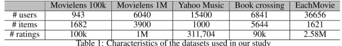
regret defined in Eq(6). Fig. 2 shows the cumulative regret of the algorithm on the synthetic data averaged over 100 runs using different size of the matrix and latent featuresK. The cumulative regret increases sub-linearly with the number of interactions and this gives us confidence that our approach works well on the synthetic dataset.
0 20 40 60 80 100 0 10 20 30 40 50 60 Iterations Cummulative Regret (a) N, M=10,K=1 0 100 200 300 400 500 0 20 40 60 80 100 120 140 160 180 200 Iterations Cummulative Regret (b) N, M=20,K=1 0 200 400 600 800 1000 0 50 100 150 200 250 300 350 400 450 Iterations Cummulative Regret (c) N, M=30,K=1 0 20 40 60 80 100 0 20 40 60 80 100 120 Iterations Cummulative Regret (d) N, M=10,K=2 0 20 40 60 80 100 0 20 40 60 80 100 120 140 Iterations Cummulative Regret (e) N, M=10,K=3
Figure 2: Cumulative regret on different sizes of the synthetic data andKaveraged over 100 runs. 5.4 Results on Real Datasets
0 2 4 6 8 10 x 104 0 5 10 15x 10 4 Iterations Cummulative Regret PTS random popular icf−20 icf−50 sgd−eps PTS−B (a) Movielens 100k 0 2 4 6 8 10 12 x 105 0 5 10 15x 10 5 Iterations Cummulative Regret PTS random popular icf−20 icf−50 sgd−eps PTS−B (b) Movielens 1M 0 0.5 1 1.5 2 2.5 3 3.5 x 10⁵ 0 1 2 3 4 5 6x 10 5 Iterations Cummulative Regret PTS random popular icf−20 icf−50 sgd−eps PTS−B (c) Yahoo Music 0 2 4 6 8 10 x 104 0 2 4 6 8 10 12 14 16 18x 10 4 Iterations Cummulative Regret PTS random popular icf−50 sgd−eps PTS−B (d) Book Crossing 0 0.5 1 1.5 2 2.5 3 x 10⁶ 0 1 2 3 4 5 6x 10 6 Iterations Cummulative Regret PTS random popular icf−20 icf−50 sgd−eps PTS−B (e) EachMovie
Figure 3: Comparison with baseline methods on five datasets.
Next, we evaluate our algorithms on five real datasets and compare them to the various baseline algorithms. We subtract the mean ratings from the data to centre it at zero. To simulate an extreme cold-start scenario we start from an empty set of user and rating. We then iterate over the datasets and assume that a random user it has arrived at time t and the system recommends an item jt
constrained to the items rated by this user in the dataset. We useK = 2for all the algorithms and use30particles for our approach. For PTS we set the value of σ2 = 0.5 andσ2
u = 1, σv2 = 1.
For PTS-B (Bayesian version, see Algo. 1 for more details), we setσ2 = 0.5and the initial shape
parameters of the Gamma distribution asα= 2andβ = 0.5. For both ICF-20 and ICF-50, we set σ2= 0.5andσ2
u= 1. Fig. 3 shows the cumulative regret of all the algorithms on the five datasets6.
Our approach performs significantly better as compared to the baseline algorithms on this diverse set of datasets. PTS-B with no parameter tuning performs slightly better than PTS and achieves the best regret. It is important to note that both PTS and PTS-B performs comparable to or even better than the “most popular” baseline despite not knowing the global popularity in advance. Note that ICF is very sensitive to the length of the initial training period; it is not clear how to set this apriori.
6
−200 0 200 400 600 800 1000 0.5 1 1.5 2 2.5 3 3.5 4 Iterations x 1000 MSE test error pmf (a) Movielens 1M 0 20 40 60 80 100 −2 −1 0 1 2 3 4 Iterations MSE RB No RB (b) RB particle filter −0.4 −0.2 0 0.2 0.4 0.6 −0.8 −0.6 −0.4 −0.2 0 0.2 0.4 0.6 ICF−20 PTS−20 PTS−100
(c) Movie feature vector
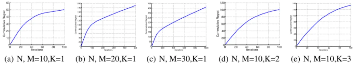
Figure 4: a) shows MSE on movielens 1M dataset, the red line is the MSE using the PMF algorithm b) shows performance of a RBPF (blue line) as compared to vanilla PF (red line) on a synthetic dataset N,M=10 and c) shows movie feature vectors for a movie with 384 ratings, the red dot is the feature vector from the ICF-20 algorithm (using 73 ratings). PTS-20 is the feature vector at 20% of the data (green dots) and PTS-100 at 100% (blue dots).
We also evaluate the performance of our model in an offline setting as follows: We divide the datasets into training and test set and iterate over the training data triplets (it, jt, rt) by pretending
thatjtis the movie recommended by our approach and update the latent factors according to RBPF.
We compute the recovered matrixRˆas the average predictionU VT from the particles at each time
step and compute the mean squared error (MSE) on the test dataset at each iteration. Unlike the batch method such as PMF which takes multiple passes over the data, our method was designed to have bounded update complexity at each iteration. We ran the algorithm using 80% data for training and the rest for testing and computed the MSE by averaging the results over 5 runs. Fig. 4(a) shows the average MSE on the movielens 1M dataset. Our MSE (0.7925) is comparable to the PMF MSE (0.7718) as shown by the red line. This demonstrates that the RBPF is performing reasonably well for matrix factorization. In addition, Fig. 4(b) shows that on the synthetic dataset, the vanilla PF suffers from degeneration as seen by the high variance. To understand the intuition why fixing the latent item featuresV as done in the ICF does not work, we perform an experiment as follows: We run the ICF algorithm on the movielens 100k dataset in which we use 20% of the data for training. At this point the ICF algorithm fixes the item featuresV and only updates the user featuresU. Next, we run our algorithm and obtain the latent features. We examined the features for one selected movie from the particles at two time intervals - one when the ICF algorithm fixes them at 20% and another one in the end as shown in the Fig. 4(c). It shows that movie features have evolved into a different location and hence fixing them early is not a good idea.
6
Related Work
Probabilistic matrix completion in a bandit setting setting was introduced in the previous work by Zhaoet al.[2]. The ICF algorithm in [2] approximates the posterior of the latent item features by a single point estimate. Several other bandit algorithms for recommendations have been proposed. Valkoet al.[14] proposed a bandit algorithm for content-based recommendations. In this approach, the features of the items are extracted from a similarity graph over the items, which is known in advance. The preferences of each user for the features are learned independently by regressing the ratings of the items from their features. The key difference in our approach is that we also learn the features of the items. In other words, we learn both the user and item factors,U andV, while [14] learn onlyU. Kocaket al.[15] combine the spectral bandit algorithm in [14] with TS. Gentile et al.[16] propose a bandit algorithm for recommendations that clusters users in an online fashion based on the similarity of their preferences. The preferences are learned by regressing the ratings of the items from their features. The features of the items are the input of the learning algorithm and they only learnU. Maillardet al.[17] study a bandit problem where the arms are partitioned into unknown clusters unlike our work which is more general.
7
Conclusion
We have proposed an efficient method for carrying out matrix factorization (M ≈U VT) in a bandit
setting. The key novelty of our approach is the combined use of Rao-Blackwellized particle filtering and Thompson sampling (PTS) in matrix factorization recommendation. This allows us to simul-taneously update the posterior probability ofU andV in an online manner while minimizing the cumulative regret. The state of the art, till now, was to either use point estimates ofUandV or use a point estimate of one of the factor (e.g.,U) and update the posterior probability of the other (V). PTS results in substantially better performance on a wide variety of real world data sets.
References
[1] Yehuda Koren, Robert Bell, and Chris Volinsky. Matrix factorization techniques for recom-mender systems.Computer, 42(8):30–37, 2009.
[2] Xiaoxue Zhao, Weinan Zhang, and Jun Wang. Interactive collaborative filtering. In Proceed-ings of the 22nd ACM international conference on Conference on information & knowledge management, pages 1411–1420. ACM, 2013.
[3] Olivier Chapelle and Lihong Li. An empirical evaluation of thompson sampling. In NIPS, pages 2249–2257, 2011.
[4] Shipra Agrawal and Navin Goyal. Thompson sampling for contextual bandits with linear payoffs. InICML (3), pages 127–135, 2013.
[5] Ruslan Salakhutdinov and Andriy Mnih. Probabilistic matrix factorization. InNIPS, volume 1, pages 2–1, 2007.
[6] Ruslan Salakhutdinov and Andriy Mnih. Bayesian probabilistic matrix factorization using markov chain monte carlo. InICML, pages 880–887, 2008.
[7] Nicolas Chopin. A sequential particle filter method for static models. Biometrika, 89(3):539– 552, 2002.
[8] Pierre Del Moral, Arnaud Doucet, and Ajay Jasra. Sequential monte carlo samplers. Journal of the Royal Statistical Society: Series B (Statistical Methodology), 68(3):411–436, 2006. [9] Arnaud Doucet, Nando De Freitas, Kevin Murphy, and Stuart Russell. Rao-blackwellised
particle filtering for dynamic bayesian networks. InProceedings of the Sixteenth conference on Uncertainty in artificial intelligence, pages 176–183. Morgan Kaufmann Publishers Inc., 2000.
[10] A. Gelman and X. L Meng. A note on bivariate distributions that are conditionally normal. Amer. Statist., 45:125–126, 1991.
[11] B. C. Arnold, E. Castillo, J. M. Sarabia, and L. Gonzalez-Vega. Multiple modes in densities with normal conditionals. Statist. Probab. Lett., 49:355–363, 2000.
[12] B. C. Arnold, E. Castillo, and J. M. Sarabia. Conditionally specified distributions: An intro-duction.Statistical Science, 16(3):249–274, 2001.
[13] Aditya Gopalan, Shie Mannor, and Yishay Mansour. Thompson sampling for complex online problems. InProceedings of The 31st International Conference on Machine Learning, pages 100–108, 2014.
[14] Michal Valko, R´emi Munos, Branislav Kveton, and Tom´aˇs Koc´ak. Spectral bandits for smooth graph functions. In31th International Conference on Machine Learning, 2014.
[15] Tom´aˇs Koc´ak, Michal Valko, R´emi Munos, and Shipra Agrawal. Spectral thompson sampling. InProceedings of the Twenty-Eighth AAAI Conference on Artificial Intelligence, 2014. [16] Claudio Gentile, Shuai Li, and Giovanni Zappella. Online clustering of bandits.arXiv preprint
arXiv:1401.8257, 2014.
[17] Odalric-Ambrym Maillard and Shie Mannor. Latent bandits. InProceedings of the 31th In-ternational Conference on Machine Learning, ICML 2014, Beijing, China, 21-26 June 2014, pages 136–144, 2014.