California State University, San Bernardino California State University, San Bernardino
CSUSB ScholarWorks
CSUSB ScholarWorks
Electronic Theses, Projects, and Dissertations Office of Graduate Studies
12-2019
THE EFFECTIVENESS OF DYNAMIC MATHEMATICAL SOFTWARE
THE EFFECTIVENESS OF DYNAMIC MATHEMATICAL SOFTWARE
IN THE INSTRUCTION OF THE UNIT CIRCLE
IN THE INSTRUCTION OF THE UNIT CIRCLE
Edward Simons
Follow this and additional works at: https://scholarworks.lib.csusb.edu/etd Part of the Science and Mathematics Education Commons
Recommended Citation Recommended Citation
Simons, Edward, "THE EFFECTIVENESS OF DYNAMIC MATHEMATICAL SOFTWARE IN THE INSTRUCTION OF THE UNIT CIRCLE" (2019). Electronic Theses, Projects, and Dissertations. 959.
THE EFFECTIVENESS OF DYNAMIC MATHEMATICAL SOFTWARE
IN THE INSTRUCTION OF THE UNIT CIRCLE
________________________
A Thesis
Presented to the
Faculty of
California State University,
San Bernardino
_________________________
In Partial Fulfillment
of the Requirements for the Degree
Master of Arts
in
Teaching: Mathematics
__________________________
by
Edward E. Simons Jr
THE EFFECTIVENESS OF DYNAMIC MATHEMATICAL SOFTWARE
IN THE INSTRUCTION OF THE UNIT CIRCLE
_________________________
A Thesis
Presented to the
Faculty of
California State University,
San Bernardino
__________________________
by
Edward E. Simons Jr
December 2019
__________________________
Approved by:
Dr. Madeleine Jetter, Committee Chair, Mathematics
Dr. Jeremy Aikin, Committee Member, Mathematics
ABSTRACT
This study is attempting to test the effectiveness of dynamic
computer models such as GeoGebra and Desmos on high school
students’ ability to understand key concepts with regards to the
introduction of unit circle and the graphing of the sine and cosine
functions.
Algebra two high school students of varying ages were chosen and
randomly placed into two groups. Both groups were given the same
pre-assessment and an identical lesson. The two groups’ only difference
occurred with the individual student practice portion of the lesson where
one group did ‘traditional’ paper and pencil practice for graphing and
solving while the other group used only computer models as their
individual practice. Both groups were then reassessed by giving the same
assessment again. Their levels of improvement were compared using
standard statistical analysis and a mean comparison test. The results
showed a statistically significant improvement in the student group that
used the dynamic models versus the group that did not use the computer.
The sample size was large enough to generate a confidence value of over
no difference between the group results and accept the hypothesis that
the student group that used the computer models improved by a
statistically significant amount. The non computer group improved by 7.7
percent while the computer aided group improved by over 49 percent.
This represented an 88 percent increase in the scores of the computer
group when compared with the control group. I was able to definitively
conclude that the dynamic software did have a significant and positive
effect on the students' learning of the unit circle.
It is hoped that this information will be used to help inform more
effective instruction for high school and college students as they learn this
topic. It also provides a strong argument for an increased emphasis on
educating teachers to become more fluent in the use of dynamic models
and software as both a demonstration tool and as an interactive tool for
their students in a variety of math levels. These results may also have
wider applications to many other math topics and math instruction in
ACKNOWLEDGEMENTS
There are many people that have contributed to my knowledge and to the
material for this paper. First, I would like to thank the student subjects, their
parents, and their teachers for allowing me into their classroom to conduct my
research and answer my questions. Second, I would like to thank my academic
advisors who have contributed so much to my thesis. These are Dr. Susan
Addington, Dr. Jeremy Aikin, and my principal advisor Dr. Madeleine Jetter. I
would especially like to thank Dr. Madeleine Jetter for her enormous patience,
dedication and constant support. Without her input and tireless dedication this
paper would not have been possible. Lastly, I would like to thank my beautiful
wife Barbara for constantly pushing me to excel and for her patience while I
TABLE OF CONTENTS
ABSTRACT……….…..……...…....iii
ACKNOWLEDGMENTS………...…….…...v
LIST OF FIGURES………....viii
CHAPTER ONE: INTRODUCTION………...…….1
History of Dynamic Software……….….…...1
Significance……….………...….…….……...3
Background ………...………….……….………...………...….4
Student Difficulties in Working with Trigonometric Functions...…...6
Training Teachers to use Dynamic Software.……...………...…………....7
Current Research…….………….………...…...8
CHAPTER TWO: OVERVIEW……..………….….…….………..16
Goals ………..………..……...17
CHAPTER THREE: METHODOLOGY…..………....…....…...…...18
Assessment, (pre and post)………....……....………...………...…...…..20
CHAPTER FOUR: PEDAGOGY……..……...………....………...…...…23
CHAPTER FIVE: STATISTICAL ANALYSIS….…...…………...………...…….29
CHAPTER SIX: CONCLUSIONS………....……...34
CHAPTER SEVEN: FUTURE RECOMMENDATIONS AND RESEARCH...39
APPENDIX A: LESSON PLAN………..………....………....…...…….41
APPENDIX B: PRE AND POST TEST………..52
APPENDIX C: ASSESSMENT SCORING RUBRIC………...56
APPENDIX D: RAW STUDENT TEST SCORES………...………….60
APPENDIX E: IRB APPROVAL LETTER………..66
DYNAMIC LESSONS USED………....………70
LIST OF FIGURES
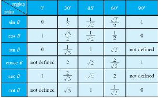
Figure 1. Trigonometry Table………...………....24
Figure 2. Screenshot of the Dynamic model of a
Sine and Cosine Generator. ………...26
Figure 3. Unit Circle Dynamic Model Generator for
Sine and Cosine Values. ……….27
Figure 4. Dynamic Model for Showing Variations in the
Period of Sine and Cosine..………..………..………...28 Figure 5. Dot Plot of the Pre Test Scores. ………...32 Figure 6. Bar Graph Comparison of Computer Groups’
Pre and Post Test Scores. ………..35
Figure 7. Bar Graph Comparison of Non Computer
Groups’ Pre and Post Test Scores. ………...35
Figure 8. Bar Graph Comparison of Pretest Scores
for the Computer vs. Non Computer Groups. ………...36 Figure 9. Bar Graph Comparison of Post Test Scores
CHAPTER ONE
INTRODUCTION
History of Dynamic Software
The history of dynamic software goes back to the mid 80’s with the
introduction of MatLab in 1984. This program was almost exclusively used at the
university level by doctoral students for research. It took nearly a decade for
dynamic math programs to be created for the use of more basic math use such
as geometry explorations. The first commercial Macintosh version of Geometer’s
Sketchpad was released in 1991. (2014, The Sketchpad Story The first
Windows version was released in 1993. It wasn’t until the release of the third
version in 1995 that widespread use of the program began and the program’s
true potential was realized. This version was designed to run on Windows 95.
This program was one of the earliest user-friendly dynamic geometry programs
but it was only available at a cost of $50. The first free programs like GeoGebra
were first introduced in 2001 and started to become more widely disseminated by
has been available to most K-12 teachers, then free dynamic software has only
been easily accessible for approximately fifteen years. Using myself as an
example of how rapidly new ideas get introduced into the K12 curriculum, I was
introduced to Geometer’s Sketchpad in my university classes in 2005 which was
within a few years of it’s introduction. There were undoubtedly others who where
introduced earlier but remember that these individuals where almost exclusively
math majors. It is much less likely that any teachers below the high school level
had any idea of the existence of, or exposure to this program. Also, the majority
of professors that were instructing the educational courses did not demonstrate
dynamic software let alone have any instructions on how to integrate it into a
math curriculum. It is easy to see how slowly the use of dynamic software is
being integrated into Mathematics curriculums due to this “educational inertia”.
There is currently no organized or mandated usage of dynamic software in
most current high school mathematics curriculums. However, it is mentioned in
the Common Core State Standards (CCSS-M as one possible method to use for
students to understand the effects of different geometric transformations. I could
predict that some sort of mandated inclusion of dynamic lessons will occur
eventually. But until then, it was only being done through the initiative of the
Math teachers that have chosen to include it as part of their normal classroom
Significance
A study where the use of dynamic software is implemented into the
curriculum by the teacher as a demonstrational tool would fit into the current
body of research by highlighting more effective methods for precalculus
instruction. This could be used by any math instructor regardless of their
proficiency with the use of dynamic software. I believe that dynamic lessons and
demonstrations could be incorporated into any math lesson at almost any level of
instruction. Arguments could be made for their effectiveness at various levels but
thousands of preconstructed models are already available on most of the free
dynamic math sites. In a recent search in GeoGebra, I found literally hundreds of
preconstructed demonstrations for “dividing fractions”. Some results were very
similar and not all were strictly covering division but this gives some idea of the
amount of free resources available from this one site. These have been made
almost exclusively by other teachers who are looking to demonstrate some math
concept in a conceptually different way. It would also help to identify any
particular concepts that may tend to more understandable if dynamic software is
used as part of the instruction.
And lastly, it is important to quantify what (if any) level of increase in
significant benefits are found in levels of student understanding, it would provide
convincing evidence that such methods should be incorporated into every
precalculus curriculum and perhaps into other levels of mathematical instruction.
Background
As the use of computers continues to infiltrate into ever more aspects of
our lives, I have observed that the use of technology is still conspicuously absent
in the majority of high school math classrooms (at least in Southern California.
There is the occasional video or perhaps an interactive link in a textbook that
very few teachers bother to explore (I know I rarely did!. Most teachers do use
computers for power points or perhaps google classroom, but that is different
from using the computer as an interactive tool to directly learn and explore a
mathematical concept. This idea of using the computer as an instructional tool
goes well beyond a simple powerpoint presentation or google search for
information.
It is my belief that all teachers need to incorporate more dynamic lessons
in their math instruction. This leads to the problem of changing the general
attitude of how math teachers approach their lessons. There are many facets to
lack of motivation of teachers or perceived benefit for teachers to use this new
technology in the classroom. If you ask a teacher if technology is beneficial to
learning, teachers will almost always answer yes. The problems start occurring
when the instruction starts and time constraints prevent teachers from ‘adding’
material to their established lessons. What teachers need to be aware of is that
dynamic software replaces more traditional techniques. If used properly, it can
save time for teachers because students can more rapidly answer questions with
the use of pre established models. According to Alsina, C., & Nelsen, R. (2006), handmade graphs on paper or chalkboard are a tedious procedure at best with arguable benefit versus the time expenditure. There is some measured benefit from these traditional methods but we now know there are more effective tools available. With today’s calculators and computers we are able to quickly graph sophisticated functions and manipulate them easily.
It is also very instructive to see the graph react as a direct result of changing the input such as using a slider that can be given any range of inputs that will immediately show the results in the graph. This is much faster than anyone could see the same results by paper and pencil graphing. I have
personally seen the confidence level of students increase in a single lesson when they are asked to graph a function using Desmos or Geogebra. And this
with graphing using the traditional methods.
Student Difficulties in Working with Trigonometric Functions
Some of the difficulties that arise for students from the introduction of graphs of trigonometric functions are that it is different in several ways from what the students have been exposed to in previous levels of math instruction.
Trigonometric functions are periodic, and it does not use any previously learned algebraic symbols. Students should have been exposed to curves that are from quadratic, cubic, exponential, and logarithmic functions but nothing that is a repeating pattern. Also, most of the key inflection points of trig functions reside at increments of pi/2 which also presents unique difficulties with many high school students attempting to graph trig functions with paper and pencil. They have almost exclusively been taught to choose small whole numbers as the best start to constructing graph. I have found that it is often the case that even when students can graph the sine and cosine functions correctly, they still have
difficulty in matching key values in the graph to the key values they are usually required to learn when introduced to the unit circle. And finally, how often do students actually use graphs or know when to use them? According to Byers,
explored. In particular, investigations using technology to capture the dynamic features of sinusoidal waveforms and the unit circle are warranted” (pg 182). It
seems logical and essential to also introduce these investigations at the high
school level as well.
Training Teachers to use Dynamic Software
Teachers tend to look upon new training as passing fads that fall in and
out of favor. The longer a teacher has been teaching the less receptive they are
to new ideas; (Makela, 1998 and for good reason. In their careers, veteran
teachers have tried dozens of varying methods that are presented by
administrators or instructors who can be somewhat less than well versed in the
demands of a high school mathematics teacher. Veteran math teachers have
usually settled on a few techniques they have found that work best for them and
produce good results in their classrooms. Those same veteran teachers are
emotionally and physically invested in those chosen methods and convincing
them of trying a new method let alone learning an entire mathematical software
packages such as Desmos or GeoGebra can be problematic. Precalculus and
trigonometry topics in particular are hundreds of years old and most teachers of
influence was incorporated into regular classroom instruction.
Current Research
Geniuses like Euler could probably visualize the infinite variations that
occur to create a moving picture in their minds. The rest of us mere mortals are
now lucky enough to have a tool available to actually see a moving picture of the
possible variations in functions like sine, cosine and tangent. But like any tool,
one needs to know the correct application for that tool, and which version of the
tool works the best for any given task. ‘Dynamic geometry software’ is available
in many forms. On a recent google search, there were 36 different programs
listed for two-dimensional geometry constructions, and eleven for three
dimensional construction.
The NCTM (National Council for the Teaching of Mathematics) indicated
that the use of varied representations are “essential elements in supporting
others. Much of the current pedagogical research relates to graphing calculators and their benefits to student learning. There is also a large body of research in
‘computer saturated’ mathematics instruction. It is widely recognized that a
varied approach (differentiated instruction) to demonstrating math concepts
allows students to choose the method(s) that fit their understanding and learning.
Consistent use of dynamic software to demonstrate math topics should be used
with the goal of getting the students to start thinking dynamically when they look at a static picture in a book or computer screen.
One attempt to do this was in a new method to teach trigonometry using
a method called MNO (Burke and Olley, 2008) M is the map of the terrain to be
covered, in this case the mathematical structure of the topic, connections and
potential problems that students might encounter. N is the narrative, the
sequencing of the lessons and activities. O is ‘orientation’, the activities which will
serve as strategies to facilitate students' engagement with the topic. The study
involved two lessons that involved competing strategies to teach trigonometric
ratios. The first used a technique called the ratio method or SohCahToa that
most math teachers are quite familiar with. If this is not familiar, SohCahToa is
an acronym that helps students remember the structure of the three basic
Soh, Cosine ϴ = hypotenuseadjacent or Cah, and Tangent ϴ = adjacentopposite or Toa. The
other lesson used two dynamic models of the unit circle. Geometer's Sketchpad
(GSP) was used to demonstrate the way the ratios are derived from a special
right triangle in the unit circle and was given to the test group. The focus of the
lesson was to compare the different strategies and the effects of GSP on both of
was not directly on whether GSP improved learning but rather, which of the
competing methods of learning trig. ratios was more effective with GSP as a part
of both lessons. Previous studies had shown the ratio method to be most
effective but the comparison was made without the use of dynamic models.
The Common Core State Standards recommend the use of dynamic
geometry software, particularly in the learning of transformations. It is unusual
that the standard is mentioning dynamic geometry as an example of what
students could do but not requiring or assessing student knowledge of
dynamic software. This is most likely due to the influence of Common Core and
the emphasis that this places on students to delve deeper and to learn ‘how’ the
answers are derived rather than just memorizing a procedure. Teachers should
teach these standards using dynamic tools. (C-GO, ‘Represent transformations
in the plane using, e.g., transparencies and geometry software; describe
points as outputs.’).
The demand for technology integrated into instruction is definitely
increasing. In a European study supported by a software company (Alexander,
et al, 2018) it reveals that universities are under increasing pressure to offer
incoming students access to state-of-the-art technology because of the increased
fees they are being asked to pay. According to the study, more than half of the
students surveyed say having access to computers and the latest software is one
of the most important factors when choosing an institution – more so than having
well-qualified and accessible lecturers. About half of the students cited increased
fees to explain their reasoning, and 89% of those starting university in 2012 “feel
entitled to a better university experience”. It is natural to assume that US
students feel similarly to our European counterparts.
I chose this topic because I have used Geometer’s Sketchpad, GeoGebra,
and Desmos software regularly in my geometry classes and with precalculus. I
was first introduced to dynamic software in my undergraduate math classes at
CSUSB and I immediately saw the benefits of it. Being able to dynamically
manipulate advanced geometry problems helped me tremendously in doing
proofs, and finding solutions. Learning the use of the software has helped me
enormously in my own math learning and I would love to be able to pass that on
the most when I teach Precalculus. I have had mostly positive feedback from
students when I ask if they feel that computer demonstrations help them to better
understand concepts rather than me at the front of the room using the
whiteboard. So there is anecdotal evidence from students and teachers that
using dynamic software increases understanding.
I have had the occasional student run with the use of Dynamic software as I
did. These students seem to thrive but whether it is directly attributable to the
software or not is debatable.
I have always had the sense that it helps but I have never done any
quantitative comparison of the benefits (to students of Sketchpad or GeoGebra.
I would like to know if this is really having an impact on student learning rather
than wasting valuable instruction time. I would also like to know what types of
mathematical concepts are best demonstrated dynamically rather than with static
methods. This is what seems to be missing in the research that I have found.
I am not unaware of the drawbacks to dynamic software. The amount of
time that is necessary to get students to log in and the initial lack of student
familiarity with the program can lead to some serious delays in actual student
learning. But an early investment of time in teaching some of the basic skills and
controls that are necessary to learn programs like Desmos or GeoGebra can pay
constructions so that they can see the basic principles involved. Moss (1997)
states that computers can make it too easy just as calculators can make knowing
multiplication less essential. Students still need to know the basics before using
the more sophisticated tools. Moss (1997) found that students’ multiplication
skills deteriorate in proportion to their dependence on calculators. Similarly,
some of the basic construction techniques such as segment bisectors, or copying
segments can be lost by relying on dynamic software too much because there
are computer tools that aid in these constructions.
In most of my searching, I found a few studies that related directly to
precalculus instruction and one was a very comprehensive study by Kan Kan
Chan and Siu Wai Leung who did research into the effectiveness of using
dynamic software.
There is a fair amount of research into the benefits of dynamic software in
K-12 math classes although much of the information is sporadic. One study that
if found was a meta-analysis of other studies that examined the effectiveness of
dynamic geometry software (DGS based upon the random effect model and
used standardized mean differences of examinations to measure outcomes.
DGS-based instruction was found to have a statistically significant positive
influence on students’ mathematical achievement in all levels of education, Chan
One paper that did measure this directly was in a study by Baharvand,
Mohsen (2001) where students used the software themselves in doing the
constructions and investigating properties. The results were markedly in support
of the dynamic software having a positive effect. In another article by Keith
Weber of Rutgers University, he states ’students need to relate diagrams of
triangles to numerical relationships and to manipulate the symbols involved in
those relationships’. This is precisely what is done when a dynamic model is
shown.
The question that follows is how much the students gain in understanding
and what level of knowledge is obtained from this. I also found a very thorough
treatment of using Geometer’s Sketchpad with geometry students and the
introductory phase of trigonometry and the learning of the basic trigonometric
ratios. Steer, de Vila and Eaton (2009). The conclusions from this study were
that 8th year students (8th grade) were able to successfully use the software to
construct triangles that represent the standard trigonometric ratios. They did not
show any significant increase in understanding when assessments were
compared to the control classrooms. I immediately wondered if any long term
data was available but was unable to find anything in my searches. This in itself
is an indication that there are serious gaps in the research of the benefits of
already existing body of research be of benefit to instructors who are reasonably
proficient in the use of Geometer's Sketchpad and GeoGebra. By increasing the
individual segments of instruction that can be shown to receive benefit from
dynamic software, the greater the emphasis will be to include these dynamic
CHAPTER TWO
OVERVIEW
The purpose of this project will be to examine the effectiveness of using
dynamic software as a demonstration tool and as an interactive tool for students
who are being introduced to the unit circle, and graphing sine and cosine. The
instructor of the experimental group will have students use dynamic software for
a minimum of 15 minutes to investigate the relationship between the unit circle
and the graph of sine and cosine. Due to time constraints, the students will use
two different dynamic models that will be limited to a one day lesson. The
primary focus of the study will be on students who are in the early stages of
learning trigonometry and more specifically, the unit circle. The groups that were
used for the study were mostly Algebra 2 students of between 14 to 17 years of
age and near the end of the second semester. All of these students should have
been introduced to trigonometric ratios the previous year when they took
geometry but there was no mention of the unit circle and little or no graphing of
trigonometric functions.
There are many applications in the various math curricula that lend
themselves to interactive models, transformational geometry, student
the trigonometric identities, the list goes on and on. I plan on trying to record
any measurable benefits or drawbacks to the employment of several of these
dynamic models in a normally paced Algebra 2 class.
Goals
The question that I would like to answer in my investigation is:
a) How Is student understanding of the unit circle, graph and its
relationship with the trigonometric functions affected when a teacher uses
dynamic demonstrations using a computer instead of static demonstrations?
b) If there is a measurable benefit of dynamic software, what portion of the
lesson benefitted the most from it?
c) If there is no measurable benefit, I would like to explore what factors
CHAPTER THREE
METHODOLOGY
This study was constructed in a pretest-posttest control grouped
half-experimental pattern. Two groups of students were studied, one group (let’s
call them group A) did not receive any interaction with dynamic models and was
taught a ‘typical’ lesson. The second group (group B) were taught the same
material with the inclusion of dynamic software (see appendix A). The treatment
group (B) used the dynamic models to replace the more typical paper and pencil
type of practice. Both groups are high school students currently enrolled in
Precalculus and Algebra two sections and were of varying ages and grade levels.
Each class that was used was divided in half for their respective groups (A and
B) by simply having every other student in each row move to one side of the
class while the remaining group moved to the other side of the classroom. This
should provide enough randomization to minimize any weighting of one group
over the other in math ability. Three of the four classroom groups were taught by
me while the fourth classroom was taught by their normal classroom teacher but
using the same lesson plan. Each class received exactly the same instruction.
Where the classes diverged were during the student practice portion of the
lesson plan which consisted of the students using paper
and pencil and trying to answer several questions that used the topic that was
taught. The treatment group was given the link to the dynamic models and
asked to explore several different topics. One example of a topic was having the
students use a slider that controlled the period and record various answers for
specific values of x (sin x).
Both groups were assessed at similar times in the curriculum. This
occurred near the end of the second semester. Most of the Algebra 2 students
should have had some exposure to the unit circle since it is now being taught in
most standard geometry curriculums. The date that the lesson was taught was
intentionally introduced to coincide with the trigonometry portion of the curriculum
in Algebra 2. A single pre-assessment was given to both groups to determine
their level of understanding. Prior student knowledge of trig functions and the
unit circle were limited to some basic lessons in the Geometry class. This would
have occurred two years prior for the students that are taking precalculus.
Precalculus students also received some additional instructions on the unit circle
Assessment (pre and post)
1.
2. Explain how you derived the x and y coordinates for each location of the unit circle.
4. How is the graph of the equation y = sin(x - π ) different from the graph of y =
sinx? What is the cause of this change?
5. Below is a graph of the function y = sin(2x). Explain (mathematically) how the graph
of this function is similar and different from the graph of y = sinx. The word bank below
is provided as a collection of terms that could be used in your explanation.
(Word Bank: Period, Amplitude, Shift, Midline, Key Values, Maximum, Minimum)
6. Define the intervals in which the sine function is increasing and decreasing in
the interval (0 to 2 ).π
7. Explain why the equation sin 2x + cos 2x = 1is true for all values of x between
0o and 360o
8. Say which is greater, sin 83 degrees or sin 175 degrees and how do you
9. Explain why the value of cosine can never be 2.
The purpose of having the students fill in the unit circle values in Question1 is to
assess their current level of knowledge and/or memorization of the unit
circle values. Question 2, ‘Explain how you derived the x and y coordinates for each location of the unit circle’, is designed to determine if they have the unit
circle values memorized or do they calculate them from special right triangles or
any other methods. Question 3 is assessing several things, first whether
students can distinguish between the graphs of sine from cosine. Second, it is
assessing their knowledge of period and amplitude. Questions 4 and 5 are to
assess how well students understand transformations of trig functions involving
shifts and compressions. Questions 6 “Define the intervals in which the sine
function is increasing and decreasing in the interval (0 to 2 )”, begins theπ
second portion of the assessment. This question is specifically targeted at
assessing the second dynamic demonstration that the test group used. We can
expect to have a significant percentage of students that will be unable to
completely fill in the unit circle values and also to incorrectly graph the sine and
cosine functions. These students will be useful in evaluating any improvement
that may occur in their ability and knowledge due to the non-dynamic versus the
CHAPTER FOUR
PEDAGOGY
The lesson plan (see appendix A that was selected was part of a
Massachusetts’ high school PreCalculus program by Douglas A Ruby (“6 Unit
Circle,” 2002 that was approved by that district and in general use. All classes
that were part of the study were able to get through about half the lesson plan.
The stoppage due to time occurred during question 4 of the lesson plan (see
appendix. Both groups progressed to where they started estimating angles on
the unit circle but the teachers were forced to cut this short in order to leave time
for the post-assessment. This balanced nicely with the test classes’ two dynamic
models. The control group followed the included paper and pencil practice that
was in the lesson while the dynamic group used two models that were available
on geogebra. The first demonstration that group B was introduced to is an
interactive model of the unit circle called “unit circle - exact values”. The students
were asked to use the software to explore the values that were preset and see
how they matched the given table of values. The hope was that they could more
quickly see how all these points on the unit circle are related to each other by
and Hostetler, section 4.2 is where the unit circle is introduced with static pictures
of the standard values similar to what is used in my pre assessment (see
question 1 of the pre assessment). In the following section, (4.3) students are
reintroduced to the 45,45,90 and 30,60,90 triangles and given the standard
values in table form (below)
Fig. 1, Trigonometry Table
Group B students were shown static pictures of the unit circle and the normal
values for 0, 30, 45, 60, and 90 degrees. They are also shown the triangle
relationships that generate these values with an interactive model in Geogebra.
This dynamic demonstration was called “unwrapping the unit circle”. It allows
tangent values change as a result. It also allows the students to click on sine
cosine or tangent and the computer will trace out the graph from 0 to 2 pi. The
hope here was to give group B a stronger visual connection from the unit circle to
the graph of the trig functions. Group A will be given a non interactive practice
with no dynamic models. Students from group B will be given an opportunity to
interact with the dynamic models.
The two groups of students will be given identical assessments (see
Appendix B and the results will be compared with special attention being paid to
any significant differences that can be attributed to the computer software. The
methods of comparison of the student data will be with the use of the statistical
analysis. This will allow me to analyze the effectiveness of the assessment and
how well it is targeted to the student group(s as well as giving me a detailed
analysis of the students’ assessment results. At the conclusion of the daily
lesson each group was given the same assessment. The recorded data was
coded to protect the students' identities. I will be looking for correlations between
the student explanations and their answers they provide on the assessment.
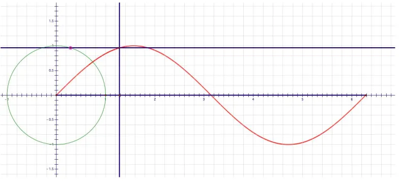
The second construction (see Figure 2 that was shown will be a similar
model of the unit circle but with the graph of the sine (or cosine function being
Fig. 2, Screenshot of the Dynamic model of a Sine and Cosine Generator
This type of activity is usually done by having students graph the key
locations of sine and cosine at 0, 90, 180, 270, and 360 degrees. It may be
beneficial to have students start the activity by doing the manual graph, and the
interactive dynamic software following to help reinforce the connections between
the two segments of the exercise. Particular emphasis will be placed upon how
the position of the circle radius and its relationship to the position of the point that
is graphing the trig function. My goal was for students to determine which values
are the dependent and independent variables.
Upon the conclusion of the two main lessons the same assessment was
given and comparisons made between the control and test groups. The pictures
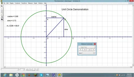
different values for sine and cosine. It is quickly apparent to the students how
the trig functions are related to the unit circle that they are controlling. One
negative aspect of this model is that the sine and cosine values are in decimal
form. It could be more helpful if they were left in radical form so that they can be
matched with special values like 21 , or . 2
√2 2 √3
Fig. 3, Unit Circle Dynamic Model Generator for Sine and Cosine Values
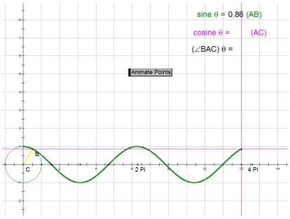
The other model below allows students to see point B travel around the
to more closely examine the demonstration and relate what is generating the x
and y values on the circle to the graph. Almost everyone quickly sees that the
circumference is the x value and the y value transfer directly from the circle to the
graph. The students are then encouraged to go back and look at the first
dynamic model where they can see the link between the special right triangles
and the sine and cosine function. This entire series of demonstrations takes
about 10 minutes.
CHAPTER FIVE
STATISTICAL DATA ANALYSIS
The body of data that was collected ended up coming from Algebra 2
students only (no precalculus students. A total of five different classrooms were
used with four of them being taught by one teacher and the remaining one taught
by me. Also recall that each classroom was randomly divided into Group A and
Group B categories by the simple expedient of having every other student move
to one side of the classroom and gathering the remaining students into the other
side. I had a total of 125 students who were included in the study because a fair
portion had to be excluded due to either missing the pre- or post-test or not
turning in the consent form. These requirements placed a large burden of
difficulty on the collection of data and will be addressed further in the final
conclusions. The statistical significance of any differences was analyzed by using
a test of the equality of two means. This was possible because the data was
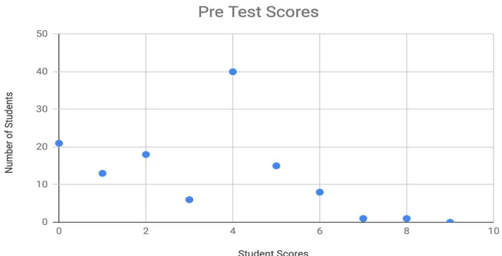
normally distributed. See graphed data below. An anomaly occurred with
student’s scoring 3 on the pretest with only 6 achieving that score out of a
possible 128 students. Also a larger than expected portion of students scored a
four. The two most commonly answered questions were questions one, with one
where many students received one point for answering “from memorization”.
There was a wide variety of different answers that contributed to the ‘4’ scores.
The question that showed the most improvement for both groups was
question 1. Many more students were able to completely fill out the unit circle or
to advance from previously not able to fill in any (zero points to more than half
correct (1 point. The question that showed the most improvement for the
computer group was question 3. More than half of that group were able to
correctly identify the graph whereas less than 20% of the non-computer group
improved on this question. More investigation on this would be necessary to
accurately determine the exact reason for this but I can surmise that the one
dynamic lesson that clearly shows the difference between the sine and cosine
graph played a significant role in this.
The mean of all students’ pretest score was 3.008. The median score was
4 of the total pretest, with the difference between the median and the mean due
to a large number of zero scores. The mean of the pretest scores for the non
computer group was 2.74 and the mean of the pretest score for the computer
Mean/Median (pre test)
Mean/Median (post test)
Percent Mean improvement
Group A (non comp)
2.74 / 2 2.95 / 3 7.7%
Group B (comp) 3.26 / 4 4.88 / 4 49.7%
This difference in pretest means, although fairly large, is not significant
because I am only trying to measure improvement from this base score (pretest.
The mean of the post test for the non computer group was 2.95 out of a possible
16 being the perfect score, so that group improved marginally. One could argue
that this was only a one day lesson so the students did not have time to absorb
or assimilate the material. The mean of the computer group post test score was
4.88 out of a possible 16, (perfect score. The non computer group had an
improvement in the mean score from the lesson of 0.21. While the treatment
group that used the dynamic models mean increase by over 1.62. We can see
from these numbers that there is a 1.41 point increase in the improvement of the
overall score where the only variable was the use or absence of dynamic
software. We can therefore note a difference in performance between student
Fig. 5, Dot Plot of the Pre Test Scores
Mean Difference Test
Let's call the test scores for the comparison (non computer students X
and the scores for the students that used the dynamic lesson Y. The mean value
that I needed was found by subtracting the post test score minus the pretest
score (Xpost - Xpre = μx ). The same was done with the test group (Ypost - Ypre =
μy). The means of each of these lists were then taken with the null hypothesis
H 0: μx - μy = 0 against the alternative hypothesis H 1: μx - μy < 0. If we assume that X and Y are independent and normally distributed with a common variance,
and if we assume respective random samples of groups X and Y, then we can
T =
X− Y√
{[(n − 1)Sx2 + (m − 1)S2Y]/(n + m − 2)}(1/n + 1/m)T has a t distribution with r = n + m - 2 degrees of freedom when H0 is true and the variances are equal. So, the hypothesis H0will be rejected in favor of H1 if the observed value of T is less than -t∝(n + m - 2). Calculating this gives
-3.12(61-64) = 15.6, so 3.12 < 15.6 and we can reject the null hypothesis.
From my data set, μx = 0.213; (the mean of the post test, no computer
minus pretest, no computer), μy = 1.609; (the mean of the post test with
computer minus pretest with computer). The variances, respectively are S2x=
1.237 and S2Y = 1.832. Using this information to determine if the differences in
means is significant with respect to the variances, I used this information to get
my T value.
=
3.12 0.90625 − 0.213CHAPTER SIX
CONCLUSIONS
The T- value of 3.12 represents a confidence interval of over 99% that we
can reject the null hypothesis and accept the hypothesis that there is a significant
improvement in the test student population. As you can see from the graphs
below, the non computer group showed a marginal positive shift while the
computer group clearly showed a significant shift from lower pretest scores to
higher post test scores. I was actually surprised by the magnitude of the
difference between the two groups. I believe more research would be useful and
beneficial but if this is shown to be a typical result of using dynamic models to
demonstrate math concepts then a much greater emphasis should be placed
upon math teacher instruction in this area.
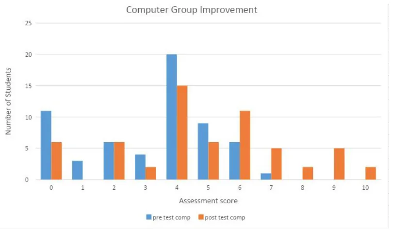
I set the following graphs up in two different ways. The first set of
graphs compares each groups’ pre and post test so that the amount of
improvement can be examined. The second set of graphs makes the
comparison between groups so readers can compare the two groups’
performance to each other based upon the pretest scores and the post test
Fig. 6, Bar Graph Comparison of Computer Groups’ Pre and Post Test Scores
Scores
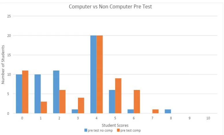
Fig. 8, Bar Graph Comparison of Pretest Scores for the Computer vs. Non
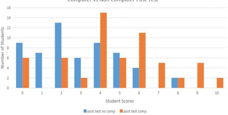
Fig. 9, Bar Graph Comparison of Post Test Scores for the Computer vs. Non
Computer Groups
Several interesting facts are apparent when examining the graphs. The
most noteworthy was the similarities in the pretest graph scores which is as
expected. When this chart is compared to the graphs of the two groups’ post test
scores the large differences are immediately apparent. The means of the pretest
non computer group and the computer group scores were 2.73 and 3.26
respectively. The post test score averages in the same order were 2.95
and 4.87. This can be seen when comparing the post test scores where the shift
from lower scores to the higher end (right can be clearly seen. One fact that I
found difficult to understand was the high number of scores of 5 in the pretest
quiz scoring rubric and the ease with which a student with marginal
understanding my get some questions correct while it would require a deeper
understanding to get closer to a score of 10. (Recall that a perfect score by the
rubric that I created would be 16)
From the pretest to the post test, the non computer group had zero scores
that were 10 and 9 respectively. The computer group had 9 and 6 from the pre
to post tests. Here again, we can see a significant drop in the number of zero
CHAPTER SEVEN
FUTURE RECOMMENDATIONS AND RESEARCH
A longer term study would be more illuminating on any benefits of dynamic
software on student learning. It would also be informative to track those students
all through their high school years. I strongly suspect that a fair percentage may
run with the use of dynamic software and start to explore on their own and use it
as a personal tool to answer homework questions and to study.
I would also like to see research at the elementary levels that incorporate
dynamic software. Such topics as fractions and basic multiplication and division
could benefit or at least provide insight into how beneficial dynamic models are to
all levels of math instruction.
This study provides strong evidence that increased usage of dynamic
software can greatly benefit student learning of the unit circle. It would be logical
to assume that dynamic software could provide benefits to other areas as well.
One specific suggestion would be in examining how the changing slope and
y-intercept in a linear equation affects the graph. This type of lesson lends itself
to computers. Other examples would be in showing how increasing dx in
integration provides greater accuracy for integral estimates using simpson’s rule
of calculus topics such a Riemann Sums. Using a slider for dx, it is readily
apparent that the sum approaches the value as dx approaches zero. The
number of possible uses are endless. The greater the body of evidence the
more widespread the usage should become which would provide benefits to all
APPENDIX A
LESSON PLAN
Unit Circle Lesson Plan
By: Douglas A. RubyClass: Pre-Calculus II
INSTRUCTIONAL OBJECTIVES:
At the end of this lesson, the student will be able to:
Date: 10/10/2002 Grades: 11/12
I. Given a real number that is an integral multiple of halves, thirds, fourths, or sixths of n, find the point on the unit circle determined by it.
2. Given a point on the unit circle that is an integral multiple of fourths, sixths, eighths, or twelfths of the distance around the circle, find the real numbers between -2n and 2n that determine that point.
3. Given any arbitrary point on the unit circle with (x, y) coordinates satisfying the equation for the circle x2 + y2 = 1, identify the 6 trigonometric functions for the angle in standard position described by a ray drawn from the origin to that point.
4. Given any arbitrary point on the unit circle with (x, y) coordinates satisfying the equation for the circle x2 + y2 = 1, find the angle in standard position described by a ray drawn from the origin to that point.
Relevant Massachusetts Curriculum Framework
PC.M. I - Describe the relationship between degree and radian measures, and use radian measure in the solution of problems, particularly problems involving angular velocity and acceleration. PC.P.3 - Demonstrate an understanding of the trigonometric functions (sine, cosine, tangent, cosecant, secant, and cotangent). Relate the functions to their geometric definitions.
MENTAL MATH-(5 Minutes)
Question 1: What are the values of the following Trigonometric Functions: a) cos -n/4 -Solution:
✓
2/2b) cos 9n/4 -Solution:
✓
2/2 c) tan 12n -Solution: 0Question 2: What does the mnemonic All Students Take Calculus stand for?
Unit Circle - Mr. Ruby
CLASS ACTIVITIES - (Note: 45 Minute Lesson Plan)
II y
(0, 0)
e
(X. 0) X
III JV
sin 0 = side hypotenuse opposite_ 0 =
cos 0 = side_ adjacent_ 0 = hypotenuse
tan 0 = side _adjacent _0 side _ opposite_ 0 y r X r y X 1 Review
If you will remember to a few days ago when we discussed Angles in Standard Position, we used the diagram to the left.
We defined an angle 0 in standard position and the six trigonometric functions related to 0. The trig functions are related to the triangle formed by using the x, and y coordinates of the ray r drawn from the origin to the point (x, y).
Therefore, the six trig functions are:
hypotenuse r csc 0 = ---''-'---=
side_ opposite_ 0 y
sec 0 = hypotenuse = r
side _adjacent_ 0 X
cot 0 = side _adjacent _ 0 X
side _opposite_ 0 y
Notice, that we can modify this diagram, by drawing a circle, whose center is the origin that intersects the ray rat point (x, y), This would look like:
JI y
(0, y)
(0, 0)
(X, 0 X
III IV
Notice also, that the equation of this circle is:
1 2 2 X + y = r
so that the length of the ray r is also the radius r of the circle. So for any point (x, y) anywhere on this circle, the same six trigonometric identities
discussed above, still holds with respect to x, y,
Unit Circle- Mr. Ruby
2. Introduction to the Unit Circle
Now suppose that instead of an arbitrary circle with a radius of r, we had what is called the unit
circle. The unit circle has a radius r of I and is defined by the equation:
So in our above looks like the diagram below.
II y
(0, y) ....
(0, 0)
III
e
(x, 0 X
IV
For the unit circle, the six trigonometric functions are:
. 0 y 1
sm = -= y csc 0 =
-1 y
X
COS 0 = -= X sec 0 = -I
X
tan 0 = l. cot 0 = -X
X
Notice, that the cos 0 and sin 0 are just the x and y coordinates of any point on the circle! Further, since tan 0 = y/x, it becomes clear that:
y sin0 x cos9
tan 0 = - = --x cos9 and cot 0 = - = --y sin9
Thus, with this simple diagram, we have completed establishing the fundamental relationship between a triangle, a circle, the six trigonometric functions, and any (x, y) point in any four
quadrants of the Cartesian plane that satisfies the equation x2 + y2 = I for the unit circle.
3. Finding Points on the Unit Circle.
11 y
(0, 0) ··· ... _ I
/
-�Sn 4
IV
Let's apply this knowledge. Example: Let's use the unit circle and our knowledge from our prior lesson on
Radians and Degrees to draw out the points on the unit circle that match certain angles. For example: If we want
to see where the angle 0 = S;r is on the unit circle, we 4
first draw the circle, then we mark the point on the circle corresponding to 0 without actually drawing the ray marking the angle in standard position. This would look like: the drawing to the left: Notice, that since the radius r = 1, the point we marked for 0 = S1r is also Sn/4 of the
Unit Circle - Mr. Ruby
way around the circle, relative to the point ( 1,0) on the initial side of the angle in standard position. (Note: Show this on the board!)
Now you try the same with a Unit circle. Draw a unit circle. Starting at the point (1,0), mark points determined by the following real numbers:
7r a)
-2 b) S
n
4 c) 2n
II
/
y
(0. 0)
d) 9,r
4 e) 13
,r 4
That is terrific. You will have three problems like this in your homework.
4. Estimating Angles on the Unit Circle
Now lets move on to estimating the real numbers between -27t and 21t that represent points on a circle relative to the point(] ,0).
II y
(0. 0) III 1! 6 X IV
Let's assume that the first marks below represent the points that are n/6, n/4, and n/3, of the way around the circle from the initial point ( 1,0). Then, as you can see, we can represent any of the points on the
Unit Circle - Mr. Ruby
Let's look at the diagram below and estimate the real numbers between -21t and 21t for the indicated points:
Try Now: How far will a point move on the unit circle, counterclockwise, in going from point A to:
ct ...
.,.
.;..�· � - ·--... ..,, " .... :i:· a) point F? n:/6:-.:
b) point H? 5n:!6
I
>;'�
'?-�-l-,,. � - .- '.,:/ J
c) point G? 4n:!3 d) point J? 11 m6
Great! Now, lets move on.
5. Using the (x, y) coordinates on the unit circle to find the six trig functions.
We already found that the definitions to for the six standard trigonometric functions are highly related to the (x, y) coordinates of any point on the unit circle as shown below:
. 0 y 0 l
Sill = -=y CSC =
-l y
X
COS 0 = - = X sec 0 = -I X
tan 0 = 2'.. x = cos.9 sin 0 cot 0 = ..:'.:. = cos ,9 y sin ,9
Further, we already know that the values of the sine and cosine for the angles in standard positions of 30°, 45°, and 60° (n/6, n/4, and n/3) for all four quadrants. Finally, let's think about what happens when we go n/2 of the way (90°) around the unit circle. What are the (x, y) values for a point on the unit circle at 0 = n/2? (0, 1) So what are the values of the sine, cosine, and tangent? (sin 0 = 1, c_os 0 = 0, tan 0 = undefined) And what are the values of the reciprocal functions cosecant, secant and cotangent? ( csc 0 = I ,sec 0 = undefined , cot 0 = 0) Great!
Now, suppose I go 5n/6 (150°) of the way around the unit circle. What is the (x, y) coordinates
for that point? (-sqrt(] )/2, ½) So what are the values of the sine, cosine, and tangent? (sin 0 = ½, cos 0= -sqrt3!2, tan 0= -l!sqrt(3)) And what are the values of the reciprocal functions cosecant, secant and cotangent? ( csc 0 = 2, sec 0 = -2/sqrt( 3) , cot 0 = -sqrt( 3 )) Great!
Unit Circle- Mr. Ruby
6. Arbitrary Points on the Unit Circle
What if the point is not one of the standard points that is a multiple of fourths (rc/2), sixths (rc/3), eighths (rc/4), or twelfths (rc/6) of the way around the unit circle? Suppose I said that the (x, y) coordinate of the point on the unit circle is ( .65, .7599342). Use your calculators to validate that it satisfies the equation for the unit circle. Then give me the six trigonometric functions for that point.
x2+ y2 = (.65;2 + (.759931?.)2 = .9999999883 -cloJt: ew>ugh!
sin 0= .759934?. csc 0= 1.31590 cos 0= .65
tan 0 = 1.16913 sec 0 cot O = = 1.53846 .85.J337
So we can find the six trigonometric functions. Let's quickly review All Students Take Calculus.
Remember, that in Quadrant I,x and y are positive. In quadrant 11,x is negative and y is positive. In quadrant Ill, x and y are both negative. In quadrant 4, x is positive and y is negative.
Therefore, we can see that All Students Take Calculus means that for the four quadrants (in oprder) All functions, Sine, Tangent, and Cosine and their reciprocals are positive. The other functions (in quadrants II, III, and IV) will be negative. Be sure to check your "sign" of your sine carefully! (pun intended).
7. Using the (x, y) coordinates on the unit circle to find the angle
The problem with knowing any arbitrary (x, y) coordinate on the unit circle and the six trig functions including their "sign" (i.e. whether they are positive or negative) is that we still don't know the angle, do we? To solve the problem of what is the angle described by an arbitrary point on the unit circle, we need to use something called inverse trigonometric functions.
Later on, we will cover the inverse trigonometric functions in more detail. But for the purposes of tonight's homework and for quizzes and tests, lets just use the functions on our calculators. There are six inverse trigonometric functions. For example, the inverse sine function is called the in x function. It is also written as the sin·' x function. The argument x of the sin·' x function is the value of sin 0. This means that arcsin xis an angle0 whose sin is x. Therefore, we can write the following equation:
0=sin·1 x
Thus, in the example above, we know that the sin 0 = .7599342. By using the sin·1 function on our calculators, we can find that:
Unit Circle - Mr. Ruby
You should see the sin-1 function on your calculators. For the following examples, find the angle of rotation in radians and degrees for each of the (x, y) points. In some cases, you will not need your calculators!
a. (0 ,I) b. (.25, .96825)
c. [
�,½)
d. (.141067, .99)0 rad, 0° 1.318 rad. 75.5234° ;T/6 rad. 3(!' 1.4293 rad. 81.8<J'
Unit Circle - Mr. Ruby
HOMEWORK (Materials):
Source:
- Bittinger and Beecher, Algebra and Trigonometry, Section 6.4, pp. 391-404
For each of the exercises 1-3, sketch a unit circle, and mark the points determined by the given real numbers:
7r
b) 3,r ) 3,r d) tr e) 11,r
I. a) - C
-4 2 4 4
7r
b) 5,r c) 11,r d) 13,r e) 23,r
2.
a)-3 6 6 6 6
II y II y
I) 2)
(0. 0) (0.0)
·-•.. I ··· ... ____ I X
III ·--� IV III IV
3. Find the real numbers M, N, P, and Q between -2n and 21t that determine each of the points
on the unit circle.
1'1'
M=2Jd3
N=571i6
'
"
N-.. ✓-"
P=51d4
,.
P=llm6 II
.,/ ....__Q
Unit Circle - Mr. Ruby
What are the (x, y) coordinates on the unit circle for the following angles? 4. rc/6 = (
J3
12, ½)5. -rc/6=(
✓
3/2,-½)6. Src/4 = ( -11-fi ,- II ,fi)
7. -Src/4=(-11,/i ,11-fi)
What are the values of the six trigonometric functions on the unit circle for the following angles? 8. rc/6
sin 0 = ½
cos 0 =
J3
/2 tan 0 = 1/✓3
9. -rc/6 sin 0 = -½ cos 0=J312 tan 0 = -1/
✓
3JO. Src/4
sin 0 = -1/ ,ti cos 0 = - l / ,fi tan 0 = I
l l. -Src/4
sin 0 = 11,fi cos 0 = -I / ,fi tan 8 = - I
12. ,423 radians sin 0 = .4/05
cos 0=.9119 tan 0 = .4502
csc 0 = 2 sec 0 = 2/
✓
3 cot 0 =✓3
csc 0 = -2
sec 0 = 2/
✓3
cot 0 = -
✓3
csc 0 =
--ti
sec 0 = --fi cot 0 = lcsc 0 = ,fi sec 0 =
--ti
cot 8 = -IUnit Circle - Mr. Ruby
For the following point, provide the six trigonometric values and the angle (in radians and degrees) outlined on the unit circle:
l3. (.823, .56804)
sin 0 = .56804 csc 0 = 1.7604
cos 0 = .823 sec 0 = 1.215 tan 0 = .6902 cot 0 =1.4489
APPENDIX B
Assessment
1.
2. Explain how you derived the x and y coordinates for each location of the unit circle.
4. How is the graph of the equation y = sin(x - π ) different from the graph of y =
sinx? What is the cause of this change?
5. Below is a graph of the function y = sin(2x). Explain (mathematically) how the graph
of this function is similar and different from the graph of y = sinx. The word bank below
is provided as a collection of terms that could be used in your explanation.
(Word Bank: Period, Amplitude, Shift, Midline, Key Values, Maximum, Minimum)
6. Define the intervals in which the sine function is increasing and decreasing in
7. Explain why the equation sin 2x + cos 2x = 1is true for all values of x between
0o and 360o
8. Say which is greater, sin 83 degrees or sin 175 degrees and how do you
know.
APPENDIX C
ASSESSMENT SCORING RUBRIC
ASSESSMENT SCORING RUBRIC
Question 1: Less than half the unit circle filled in correctly - 0 points
Between half correct and totally correct - 1 point
Completely filled in (correctly) - 2 points
Any type of mention of special right triangles or “from memorization”
but not a complete demonstration of their understanding or an
explanation of their reasoning. If a student answer “from memorization, they
needed to have scored at least on point on question 1 - 1 point
An explanation that was clearly understood and demonstrated a level
of deeper knowledge of the origin of the values. - 2 points
Question 3: No answer or any non Cosine answer with no shift. - 0 points
Any Cosine (or shifted Sine) answer with incorrect amplitude. - 1 Point
A Cosine (or shifted Sine) answer with a correct amplitude - 2 points
Question 4: An incorrect explanation of the difference and incorrect cause -
0 points
A correct explanation of the difference but incorrect cause or incorrect
explanation with correct cause - 1 point
Correct explanation and cause - 2 points
Question 5: No correctly explained differences or similarities and key words
used incorrectly - 0 points
Either one correct similarity or difference with at least one correct use
of a wordbank word - 1 point
A correct similarity and a correct difference where both are explained
Question 6: No correct explanation of any intervals - 0 points
Partially correct explanation with at least one interval correct - 1 points
All intervals correct with an explanation that is relevant - 2 points
Question 7: No correct explanation - 0 points
A partially correct explanation that demonstrates either some
understanding of the max and min values of sine and cosine or with
the Pythagorean theorem. - 1 point
An explanation that is clearly understandable and demonstrates
knowledge of both the Pythagorean theorem and the values of sine
and cosine- 2 points
Question 8: Incorrect with no or incorrect explanation - 0 points
Correct with no or incorrect explanation - 1 points
Correct with a correct explanation - 2 points
Question 9: No explanation or one that is nonsensical. - 0 points
A partially correct but incomplete explanation with no mention of the
Pythagorean identity in question 7. - 1 point
A complete explanation that clearly shows depth of knowledge of sine
and cosine and how they would evaluation in the Pythagorean identity