www.nat-hazards-earth-syst-sci.net/15/2227/2015/ doi:10.5194/nhess-15-2227-2015
© Author(s) 2015. CC Attribution 3.0 License.
Three-dimensional slope stability problem with a surcharge load
Y. M. Cheng1, N. Li1, and X. Q. Yang2
1Department of Civil and Environmental Engineering, Hong Kong Polytechnic University, Hong Kong, China 2Building and Construction Department, Guangdong University of Technology, Guangzhou, China
Correspondence to: Y. M. Cheng ([email protected])
Received: 15 January 2015 – Published in Nat. Hazards Earth Syst. Sci. Discuss.: 11 February 2015 Revised: 31 August 2015 – Accepted: 3 September 2015 – Published: 8 October 2015
Abstract. A semi-analytical solution for the three-dimensional stability analysis of the ultimate uniform patched load on top of a slope is developed by the limit analysis using kinematically admissible failure mechanisms. The failure mechanism which is assumed in the analytical solution is verified by three-dimensional strength reduction analyses and laboratory model test. Furthermore, the pro-posed method and the results are further compared with some published results for illustrating the applicability of the proposed failure mechanism.
1 Introduction
Many practical geotechnical problems are three-dimensional in nature, yet two-dimensional plane-strain analysis is com-monly used for simplicity of analysis. This pertain to prob-lems as natural slopes, cut slopes and fill slopes for which the failure regions usually have finite dimensions, and the actual problems are far from the plane strain condition. For two-dimensional slope stability by the limit equilibrium method, the factor of safety is based on the equilibrium of discrete slices (Bishop, 1955; Morgenstern and Price, 1965; Spencer, 1967; Janbu, 1973). Two-dimensional analyses, though help-ful for designing most of the slopes and embankments, are not applicable to slopes with local loads, which may lead to conservative design by assuming loads of an infinite extent through 2-D methods. Cheng et al. (2007) has demonstrated that the strength reduction method is similar to the limit equi-librium method in most cases, and the strength reduction method will also be adopted for comparisons in this study. Hong Kong has a long history of tragic landslides with sig-nificant loss of life and property damage. From government’s record, more than 470 people died as a result of slope failures
since 1947. Currently, the Hong Kong Government is spend-ing about USD 130 million each year for slope stabiliza-tion, and such stabilization works have launched for about 40 years. More critical slope failure problems are being faced the Chinese Government, and there are various types of slope research underway in Hong Kong, China and many other ar-eas. The present work is part of the continuous research pro-gramme by the authors (Cheng et al., 2013b; Li and Cheng, 2015), which include the use of innovative slope stabilization methods, debris flow flume and large-scale tests, advanced theory and design practice useful for both researchers and engineers, for both natural and reinforced slopes. Slopes in front of bridge abutment are very common in many coun-tries. Currently, these slopes are commonly analyzed as two-dimensional problems, and the present work is devoted to this problem with an aim of providing a more realistic tool (validated by experiments and numerical analysis) suitable for the engineers to use.
and Wei et al. (2009) have carried out a detailed study about three-dimensional slope stability analysis using strength re-duction method (SRM).
The safety factor for a three-dimensional problem is defined in the same way as for the corresponding two-dimensional problems:
c=cs/ k (1)
tanϕ=tanϕs/ k, (2)
wherecs andϕsare soil cohesion strength and internal fric-tion angle,kis the traditional safety factor, andcandφare the mobilized cohesive strength and internal friction angle, respectively. In most of the previous works based on the limit analysis, the failure mass is divided into several blocks with velocity discontinuity planes along the discontinuity surface and energy balance is applied (Chen, 1975).
Implementation of the upper bound theorem is generally carried out as follows. (a) First, a kinematically admissi-ble velocity field is constructed. No separations or overlaps should occur anywhere in the soil mass. (b) Second, two rates are then calculated: the rate of internal energy dissi-pation along the slip surface and discontinuities that separate the various velocity regions, and the rate of work done by all the external forces, including gravity forces, surface tractions and pore water pressures. (c) Third, the above two rates are set to be equal. The resulting equation, called energy–work balance equation, is solved for the applied load on the soil mass. This load would be equal to or greater than the true collapse load (Cheng and Lau, 2013).
It should be mentioned that discontinuous fields of veloc-ity is used in applying upper bound theorem. Surfaces of ve-locity discontinuity are clearly possible, provided the energy dissipation is properly computed. For instance, rigid-body sliding of one part of the body against the other part is a well-known example. This discontinuous surface should be regarded as the limiting case of continuous velocity fields, in which one or more velocity components change very rapidly across a narrow transition layer, which is replaced by a dis-continuity surface as a matter of convenience. Discontinuous velocity fields not only prove convenient but often are con-tained in actual collapse mode or mechanism (Chen and Liu, 1990).
This approach is acceptable for a two-dimensional anal-ysis, but a realistic three-dimensional failure mechanism should have a radial shear zone which is difficult to be mod-elled by wedges. Chen et al. (2003) overcome this limitation by the use of many small rigid elements and nonlinear pro-gramming technique for the minimization analysis, but this method requires very long computer time in the optimization process, and the location of the global minimum is not easily achieved.
In this paper, semi-analytical solutions for a patched uni-form distributed load acting on or below the top surface of a slope are developed. This problem can also be viewed as a
bearing capacity problem as well as a slope stability problem. The failure mechanism presented in this study is a more rea-sonable mechanism based on the kinematically admissible approach of a typical bearing capacity problem. It is a further development of the works based on some of the above re-searches by using a more reasonable three-dimensional radial shear failure zone through which other three-dimensional failure wedges are connected together with, and a solution can be obtained within very short time as the semi-analytical expressions are available. The present solutions have given good results when compared with some previous studies and a laboratory test shown in Fig. 6, also demonstrated by Li and Cheng (2015). The laboratory test has also revealed some interesting progressive failure phenomenon and deformation characteristic for this slope failure problem.
2 Theoretical background of the 3-D failure mechanism
Kinematically admissible velocity fields used in the upper bounds analysis usually have a distinct physical interpre-tation which is associated with the true collapse mecha-nisms known from experiments and practical experience. The present failure mechanism complies with the require-ments in limit analysis and is similar to that as found from laboratory tests which will be illustrated in a later section. Stress fields used in the lower-bound approach, however, are constructed without a clear relation to the real stress fields, other than the stress boundary conditions. Moreover, most problems involve a semi-infinite half-space, and the exten-sion of the stress field into the half-space is either cumber-some or appears to be impossible (Michalowski, 1989). For general three-dimensional problems, the construction of an admissible stress field is very difficult, and only very few cases are successfully solved by the lower bound approach. As a result, only the upper-bound kinematical admissible ap-proach is commonly adopted for solving such problems.
merge with the ground surface. This lateral failure mecha-nism can be viewed as the effect of the Poisson’s ratio which generate lateral stress and hence lateral failure. The details and the geometry of the failure mechanism will be discussed in details in the following sections.
3 Three-dimensional slope failure of a slope with patched load on the top surface (D=0 m)
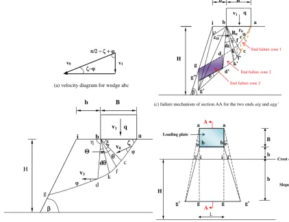
A simple three-dimensional slope failure mechanism with zero embedment depth patch load (D=0 m) is shown in Fig. 1. The failure mechanism is asymmetric as there is slope in front of the patch load, and the failure mechanism is con-trolled by angle ζ andξ which are to be determined. The surface between the footing and the soil is assumed to be smooth in the present study. Figure 1b is the failure mecha-nism at the section through the applied load, while the end effects are shown in Fig. 1c, which is the failure zone nor-mal to the section in Fig. 1b and illustrated as agg’ zone on the left and right sides of Fig. 1d. The bird view of the three-dimensional failure mechanism is shown in Fig. 1d. The total works done are calculated as below.
3.1 Rate of work done produced along load lengthL
In the following analysis, some of the geometry determina-tions are given in the Appendix while the main theme about the energy balance will be discussed. Based on Fig. 1b, the resistance rate of work doneP dissipated by the cohesionc along the velocity discontinuity planeac·Lis given as PR1=c·ac·L·v0cosϕ, (3) whereac=Bsinξ /sin(ζ+ξ )andr0=bc=Bsinζ /sin(ζ+
ξ ),B is the width of the footing andLis the length of the footing normal to the section as shown in Fig. 1b but exclud-ing the two end effects. Resistance rate of work done dissi-pated in the radial shear zone bcd is written as (see Chen, 1975)
PR2=cv0r0L
exp(22tanϕ)−1
tanϕ . (4)
Resistance rate of work done dissipated by cohesioncalong the velocity discontinuity planedg·Lis given by
PR3=c·dg·L·v3cosϕ, (5)
in whichv3=v0exp(2tanϕ), andbd=r0exp(2tanϕ). As shown in Fig. 1b, point b is taken as the reference point (0, 0, 0) of the coordinates axes, and positive directions are pointing left and downward. The rate of work done produced by the external pressure q on the top of the slope is expressed as
PD1=qBLv1. (6)
The rate of work done produced by the weight of the wedge abcis written as
PD2=Wabcv0sin(ζ−ϕ), (7)
whereWabc=γ2ac·B·Lsinζ. The rate of work done
pro-duced by the weight of the radial shear zonebcdis given as (see Chen, 1975)
PD3=γ
2
2
Z
0
r2Lvcos(θ+ξ )dθ
=γ
2r 2 0Lv0
exp(32tanϕ)[sin(2+ξ )+3 tanϕcos(2+ξ )] −sinξ−3 tanϕcosξ
1+9tan2ϕ
. (8)
The rate of work done dissipated by the weight of the wedge bdgiis formulated as (refer to Eq. (A1)–(A4) of Appendix) PD4=Wbdgi ·v3cos(180◦−η) (9)
Wbdgi=γ L(Sbig+Sbdg). (10)
3.2 Rate of work done produced at the two end-failure zones of the footing
A lateral wedge, log-spiral, wedge failure mechanism has been assumed in the present study, and the rate of work done will be considered here. The overall results based on the present mechanism are found to be better than some other published results which will be shown later.
1. End failure zone 1 (correspond to side of failure below foundation at mid-section, illustrated as plane acc’ in Fig. 1c)
As shown in Fig. 1c,cc0 is a horizontal line normal to the planeabc. In order to ensure that the sliding veloc-ity of the soil mass of the end-failure zone 1 is equal tov0, the angle betweenacand should be equal toφ, therefore,cc0=r0tanϕ, r0=ac (refer to Eq. (A5) of the Appendix). The rate of work done by the velocity discontinuity planeacc0is then expressed as
PRE1=c·Sacc0 ·v0cosϕ, (11) whereSacc0=1
2ac·cc
0. The rate of work done produced
by the weight of the wedgeabc−c0is expressed as
PDE1=Wabc−c0 ·v0sin(ζ−ϕ). (12)
v1
v0
(a) velocity diagram for wedge abc
(b) failure mechanism (excluding the two ends) v3
i b a
v1 q
v0
g
d k f
c H
b B
d
(c) failure mechanism of section AA for the two ends aig and agg’
(d) three-dimensional failure mechanism on plan
g
g’ g”
a b
v1 q
d’ k’f’
c ’ H
d k
fc R0 r0 i
i’
b B
H
g’ g g g’
h b B
a a
b b
i’ i i i’
d
H
L
A
A
Crest of slope Loading plate
Slope surface End failure zone 3
End failure zone 1
End failure zone 2
Figure 1. Three-dimensional failure mechanism for slope problem with a patch load.
a. Velocity discontinuity curve plane bc0d0 (refer to Eq. (A8) of the Appendix)
The resistance rate of work done produced by c along the velocity discontinuity planebc0d0 is in-tegrated as
PRE2=
εH R
0
c·Sbf0k0·vcosϕ·dθ=1 2cv0R
2 0
cosϕ 2
R
0
exp(3θtanϕ)dθ
= cosϕ
6 tanϕcv0R
2
0[exp(32tanϕ)−1]
. (13)
b. Velocity discontinuity plane cc0d0d (refer to Eqs. (A9)– (A10) of the Appendix)
The resistance rate of work done produced by the velocity discontinuity areacc0d0dis obtained as
PRE3= 2
Z
0
Sf f0k0k·v·ccosϕdθ
=1
3r 2
0v0c[exp(32tanϕ)−1] (14) .
c. Radial shear zoneb−cc0d0d (refer to Eq. (A11) of the Appendix)
Dissipated rate of work done produced in the radial zone is given as
PRE4= 2
R
0
Sbf f0·c·vdθ= 1 2r
2 0cv0 tanϕ
2
R
0
exp(3θtanϕ)dθ
=1
6r 2
0cv0[exp(32tanϕ)−1]
(15)
d. Weight of the radial zone b−cc0d0d(0≤θ≤2) (refer to Eq. (A12) of the Appendix)
The driving rate of work done produced by the weight of the wedge is expressed as
PDE2=
2 R
0
Wb−f f0k0k·vcos(ξ+θ )dθ
=γ 3r
2 0R0v0sinϕ
exp[42tanϕ][sin(2+ξ )+4 tanϕcos(2+ξ )] −sinξ−4 tanϕcosξ
1+16tan2ϕ
.
(16) 3. End failure zone 3 (correspond to the wedge zone out-side the log-spiral zone, illustrated as plane dd’g”g in Fig. 1c)
a. Resistance rate of work done produced bycalong the velocity discontinuity plane is then obtained as (refer to Eq. (A13) of the Appendix)
PRE5=c·Sdd0g0g·v3cosϕ. (17) b. Velocity discontinuity plane bd0g0i0 (refer to
Eqs. (A14)–(A17) of the Appendix)
The resistance rate of work done produced bycalong the velocity discontinuity plane is written as
PRE6=c·(Sbd0g0+Sbg0i0)·v3cosϕ. (18) c. Wedgeb−dd0g0g
Weight of the wedgeb−dd0g0gis expressed as Wb−dd0g0g=
γ
3Sdd0g0g·bdcosϕ. (19) . The corresponding resistance rate of work done pro-duced by the weight of wedge is obtained as
PDE3=Wb−dd0g0g·v3cos(180◦−η) (20) d. Wedgeb−gg0i0i
Weight of the wedgeb−gg0i0iis given by Wb−gg0i0i=
γ
3 ·Sgg0i0i·bsinβ. (21) in which Sgg0i0i =1
2gi·(yi0+yg0), gi=
q
(xg−xi)2+(zg−zi)2.
Then resistance rate of work done produced by the weight of the wedge is
PDE4=Wb−gg0i0i·v3cos(180◦−η). (22)
The total resistance rate of work done of the failure mechanism shown in Fig. 1 is expressed as
PR=PR1 +PR2+PR3+2(PRE1 +PRE2
+PRE3+PRE4+PRE5 +PRE6). (23) The total driving rate of work done is obtained as
PD=PD1+PD2+PD3+PD4+2(PDE1
+PDE2+PDE3+PDE4). (24)
By means of Eqs. (1) and (2), the safety factor k are obtained by means of a simple looping method starting ask=1.0 in the initial trial then trying with differentk until the following equation is satisfied:
PR−PD=f (ζ, ξ, η)=0, (25) where the anglesζ,ξ andη related to thek value are the critical failure angles,ζcr,ξcr andηcr;f is a yield function and plastic flow can occur only when the yield function is equal to 0 (Chen and Liu, 1990). Various techniques can be used to solve Eq. (25) for which there are four variables (3 angles plusk). Instead of using ad-vanced numerical technique for this problem, the au-thors have chosen to use a very simple looping method. Each variable is looped within a specified and accept-able range, and the rate of increment of the angle is generally kept to be 0.5◦initially. During the solution of nonlinear Eq. (25), it is found that the solution is very sensitive to the parameters near to the critical solution. A small change of even 0.5◦can sometimes have a
no-ticeable effect to the solution of Eq. (25) under such condition. Regarding that, a small interval of 0.2◦ is chosen in the present study. The advantage of the loop-ing technique is that the sensitivity of the solution algo-rithm can be avoided simply by a small interval of 0.2◦ instead of using special treatment in the numerical algo-rithm. Even with such a small interval in the search for the critical solution, the solution time is extremely fast and is acceptable.
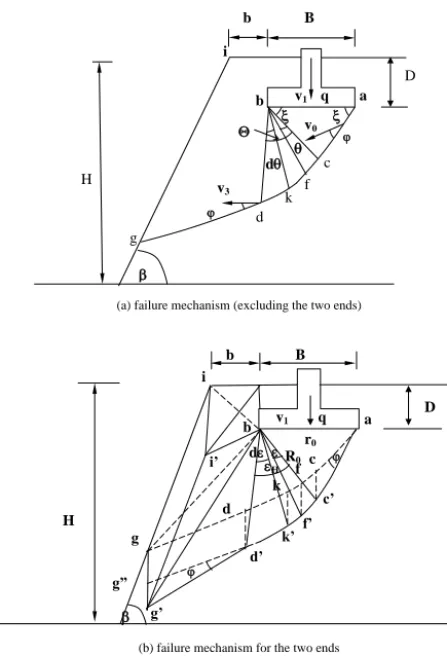
4 Three-dimensional slope failure with an embedded patched load (D> 0 m)
(a) failure mechanism (excluding the two ends)
(b) failure mechanism for the two ends
v3
i
b v1 q a
v0
g
d k f
c H
b B
d
D
g
g’ g”
a
b v1 q
d’ k’f’
c’ H
d k
f c R0
r0 i
i’
b B
D
d
H
Figure 2. Three-dimensional failure mechanism for slope with
buried patch load.
4.1 Rate of work done produced along footing lengthL
– Resistance rate of work done dissipated by cohesionc along velocity discontinuity planedg·Lis calculated by (refer to Eqs. (A18)–(A20) of the Appendix)
PR3=c·dg·L·v3cosϕ (26) in which v3=v0exp(2tanϕ), and bd=
r0exp(2tanϕ).
– Resistance rate of work done is produced by the weight of the wedgebdgih(refer to Eq. (A21a)–(c) of the Ap-pendix):
Wbdgih=γ·L·Sbdgih (27)
Then, the rate of work done produced by the weight of the wedge bdgih is given as (refer to Eqs. (A23)–(A25) of the Appendix)
PD4=Wbdgih·v3cos(180◦−η), (28)
Other items such asPR1, PR2andPD1∼PD3are similar to those given in the previous section and will not be repeated here.
4.2 Rate of work done produced at two failure ends of the buried load
a. Velocity discontinuity plane bd0g0i0 (refer to Eqs. (A22)–(A26), Eq. (A27) of the Appendix) For the velocity discontinuity planebd0g0, it is similar to the previous case except that
bi0=
q
xi20+yi20+zi20 (29) The resistance rate of work done produced bycalong the velocity discontinuity planebd0g0i0is also given by Eq. (18).
b. Resistance rate of work done produced by the tensile failure planebhi0
Area of the tensile failure planebhi0is expressed as Sbhi0=
1 2D·hi
0
, (30)
in whichhi0=
q
b2+y2
i0. Usually, the tensile strength of soil mass can be taken as (1/4–1.0)c(Baker, 1981; Bagge, 1985). Calculation as shown in later part of this paper will demonstrate that the tensile strength of soil mass has only a small effect on the safety factor, so it is assumed to be equal to c/3 in the present study (any other value can be obtained easily by a very sim-ple modification of Eq. 31). As the tensile direction is along the direction of velocityv3, the corresponding re-sistance rate of work done produced by the tensile fail-ure plane is written as
PRE7=c·Sbhi0·v3/3, (31) c. Driving rate of work done produced by wedges b−
dd0g0g,b−ii0g0gandb−hii0
Then driving rate of work done produced by the weight of these wedges is expressed as
PDE3=(Wb−dd0g0gi+Wb−ii0g0g+Wb−hii0)
Other itemsWRE1•∼WRE5•andWDE1•∼WDE2• are similar to the case forD=0 m and will not be repeated here. Referring to Fig. 2, the total resistance rate of work done is expressed as
PR=PR1+PR2+PR3 +2(PRE1+PRE2
+PRE3 +PRE4+PRE5+PRE6+PRE7). (33) The total driving rate of work done of Fig. 2 is obtained as
PD=PD1+PD2+PD3+PD4
+2(PDE1+PDE2+PDE3). (34)
kwill be obtained by setting Eq. (33) equals Eq. (34).
5 Comparison of the authors’ method with other analytical solutions
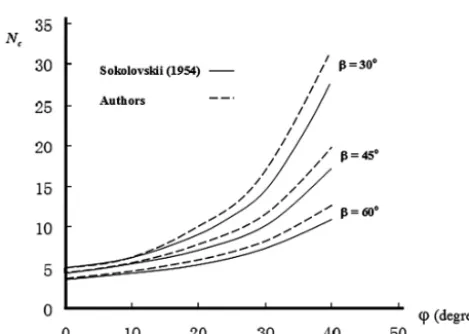
Referring to Fig. 1, when b=0, based on the well-known slip-line solutions by Sokolovskii (1960), the closed form solution of bearing capacity factor Nc to the ultimate bear-ing pressurequ(qu=cNc+qNq)for a weightless soil mass
is given by
Nc=c·cotϕntan2(45◦+ϕ
2)exp[(π−2β)tanϕ] −1
o
. (35) For a two-dimensional plane problem with weightless soil mass,Ncvalues for different slope angles are calculated by using Eq. (25). Safety factorkis set to 1.0, and an arbitrary value ofc(10 kPa used by the author) is used in Eq. (25) for a givenϕ. The value ofquis adjusted by trial and error until Eq. (25) is satisfied. Sinceq which is the surcharge outside the foundation is 0,Ncis hence determined. The same result can also be determined Eq. (35), and the results are shown in Fig 3. The general trends for the variations of theNcand angle friction, which was predicted by both of the methods, are similar, butNcvalues by Eq. (25) are only slightly larger than theNcvalues by Eq. (35). This indicates that the three-dimensional failure mechanism of Fig. 1 is a reasonable up-per bound solution for two-dimensional analysis.
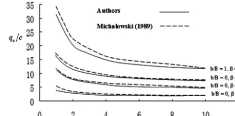
Further comparison has been carried out for a three-dimensional slope stability analyses with the following soil properties (c=20 kN m−2,ϕ=20◦andγ =20 kN m−3)and slope geometry (B=2 m,b=1 m, D=0 m andH=6 m). The results of the dimensionless limit pressure qu/c val-ues with different L/Bvalues are illustrated in Fig. 4, and the results by the authors are slightly smaller than those by Michalowski (1989). According to the upper bound theorem, the smaller result obtained by the authors will be the bet-ter result. Since both the present approach and the one by Michalowski (1989) are upper bound approach with only mi-nor differences in the failure mechanism, slightly smaller re-sults by the authors imply the failure mechanism as adopted
Figure 3. Comparison of present results with upper-bound solutions
by Michalowski (1989).
is closer to the true failure mechanism. The ultimate pres-sures decrease with the increase in L/B ratio. Until the L/Bvalue greater than 5, the normalized ultimate pressures are not sensitive to the variations of theL/B values. Such trends are shown in both of the methods. This indicates that the effect of the patched pressure on the top surface of the slope will increases rapidly as the dimensionL/Bratio is re-duced, especially forL/B< 5. Moreover, the ultimate pres-sures given by the authors are slightly lower than the ulti-mate pressure given by Michalowski (1989), which required more parameters in the formulations. According to the up-per bound theorem in plasticity (Chen, 1975), the present three-dimensional failure modes are more reasonable and more critical than that by Michalowski (1989), as the ulti-mate pressure from the present formulation is smaller than that by Michalowski (1989). Compared with other previous works, the present results can give better predictions for the ultimate local pressure on the top surface of the slope.
As mentioned previously, the tensile strength of soil has very little impact on the results of analysis. The authors have tried to change the tensile strength equal to 1/3c to 1/2c in the analysis and have found that the results in Fig. 3 are nearly not affected, particularly whenβis small (below 30◦).
Whenβis large, the changes in the results are limited to less than 3 % in general. Regarding of that, the results in Fig. 3 can be used directly in general without any practical needs for refinement.
6 Verification by numerical analysis
Figure 4. Comparison of Ncvalues between Sokolovskii method and authors’ method.
the safety factork is increased as theL/B ratios decreased gradually, which is a typical illustration of the importance of three-dimensional effects. WhenL/B=1.0, the failure sur-face from SRM is still a basically two-dimensional mecha-nism which is illustrated in Fig. 5, and the factor of safety from SRM is only 1.71 which is far from 2.084 from the present 3-D failure mechanism (as shown in Fig. 1). Unless the loading is large enough, only a 2-D failure mechanism will appear in 3-D SRM which is not realistic, and this is the limitation of the SRM, and the present formulation is better than the SRM in this respect. It is found that whenL/B ra-tio is great so that the failure mechanism is approaching a two-dimensional failure, the results from Eq. (25) is virtually the same as the results from three-dimensional SRM. When L/Bratio is small, there are however more significant differ-ences between the present failure mechanism and the SRM. The shear strain contour at the ultimate state was shown in Fig. 5. There is shear strain concentration, i.e. a shear band from the top to the toe of the slope.
7 Verification by laboratory model tests
A laboratory test complying exactly with the present prob-lem as shown in Fig. 6 has been performed for the verifica-tion of the proposed method. A hydraulic jack applies a local load on top of a 0.8 m high 65◦inclined slope. The soil used for the model slope is classified as highly permeable poorly graded river sand. The unit weight and the relative density are γ =15.75 kN m−3and 0.55, the relative density is defined as the ratio of (actual density-loosest density) against (highest density-loosest density) which is a dimensionless index for soil. Shear strength parameters (c0=7 kPa andφ’=35◦) of the soil was determined by means of consolidated drained tri-axial test. The depth, breadth and height of the soil tank are 1.5, 1.85 and 1.2 m respectively. The soil is compacted by an electric compactor with a 0.2 m×0.2 m wooden end plate.
Figure 5. Failure mechanism for L/B=1.0 by SRM (shear strain distribution).
Figure 6. Basic setup of the laboratory test.
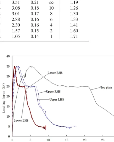
Five linear variable differential transducers (LVDTs) are set up to measure the displacement of soil at different locations; the upper right (RHS), upper left (LHS), lower right (RHS) and lower left (LHS) are shown in Fig. 7, and the displace-ments at different vertical loads are monitored up to failure as shown in 8. The two pairs of transducers on the slope sur-face are placed symmetrically with a horizontal spacing of 300 mm. The first and second pairs of transducers are placed at vertical distances of 150 mm and 450 mm from the top of the slope, respectively.
Table 1. Safety factors and geometric parameters (Example 1 and geometry of failure mass) forq=100 kPa.
k ζcr(◦) ξcr(◦) ηcr(◦) h(m) cc0(m) gg0(m) ii0(m) L/B kfrom SRM
1.120 69.0 68.3 94.75 6.00 0.88 3.51 0.21 ∞ 1.19
1.278 67.8 67.1 97.75 6.00 0.74 3.08 0.18 10 1.26
1.311 67.3 67.0 98.25 6.00 0.72 3.01 0.17 8 1.30
1.368 67.0 66.8 99.25 6.00 0.67 2.88 0.16 6 1.33
1.466 64.6 64.3 97.75 4.97 0.57 2.30 0.16 4 1.41
1.706 60.8 60.5 95.00 3.72 0.43 1.57 0.15 2 1.60
2.080 57.0 56.8 92.00 2.83 0.32 1.05 0.14 1 1.71
Figure 7. LVDT at top and sloping face of the model test.
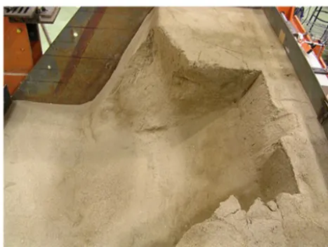
as shown in Fig. 8. As a result, the ultimate bearing capac-ity of the slope under the current soil properties, geometrical conditions and boundary conditions is 181.2 kPa, which re-sults in a factor safety 1.021 with the present method. This value is very close to 1.0, which demonstrates that the result is reasonable. For the slope surface, the corresponding dis-placement at the maximum pressure is about 2 and 1 mm at top and bottom of the slope respectively. Beyond the peak load, the applied load decreases with the increasing jack dis-placement. It is clear that the displacements of the slope are basically symmetrical. The failure surface of the present test is shown in Figs. 9 and 10, and the sectional view at the mid-dle of the failure mass is shown in Fig. 11. In Fig. 8, after the maximum load is achieved, the load will decrease with in-creasing displacement. At this stage, the local triangular fail-ure zone is fully developed, while the failfail-ure zones at the two ends of the plate are not clearly formed. When the applied load has decreased down to about 25 kN, the load maintained constant for a while and the failure zones at the two ends are becoming visually clear. When the displacements are further increased, the applied load decreases further, and the failure zone propagate towards the slope surface until the failure sur-face as shown in Fig. 10 is obtained. This three-dimensional failure mechanism as measured from the model test is basi-cally similar to that as given in the semi-analytical approach, and the prediction of the factor of safety from the present theory is also satisfactory.
For this test, there are several interesting phenomena worth discussing. The failure profile and cracks are firstly initiated beneath the footing as shown in Fig. 9, which is a typical bearing capacity/slope stability failure with a triangular
fail-Figure 8. Loading force against the displacement of slope surface.
Figure 9. Slope failure beneath bearing plate.
Figure 10. Global three-dimensional slope failure.
Fig. 10. It is observed that the failure mechanism of the phys-ical model test is hence a local triangular failure beneath the bearing plate, and the failure surface propagates towards the slope surface until a failure mechanism is formed. The failure profile matched reasonably well with that as predicted from the present formulation as shown in Fig. 11, and is also in compliance with that as developed by Cheng and Au (2005) using the slip line method. In addition, the prediction of the factor of safety is also close to the back analysis result of the laboratory test. Regarding the difficulty in ensuring complete uniformity for the compaction of the model slope, the small discrepancy between the predicted and measured failure pro-files as shown in Fig. 11 can be considered as acceptable.
8 Discussion and conclusions
Based on the upper bound theorem of limit analysis, a three-dimensional slope stability problem with a patched uniform distributed load on the top surface are investigated. The semi-analytical method has demonstrated that the present failure mechanisms are reasonable in predicting the bearing capac-ity under a patched load on the top surface of slope, which is commonly found for bridge abutment foundation. Further-more, combined with the traditional safety factork, the al-lowable load on the top surface of the slope can be obtained by a simple looping method (using Excel or any computer language). The search for the critical factor of safety is just several seconds, which is much faster than that by the SRM which requires about half to 1 day for a complete analysis (and about half a day to set up the computer model for an experienced user), but the results from the proposed analysis is very close to that from the tedious analysis using SRM.
Figure 11. Comparisons between the measure and the predicted
failure surface profile at mid-section of failure.
The present formulations are the further extension of pre-vious works, with slightly improved results and more versa-tile for both surface patch load or buried patch load. Based on the model test and the SRM analysis, it is clear that the present work can be used by engineers for routine analysis and design, and it can provide fast and reliable solution suit-able for many practical problems.
Appendix A: Geometrical relations
A1 Three-dimensional slope failure of a slope with patched load on the top surface (D=0 m) A1.1 Along footing lengthL
If the coordinate of pointbisxb=0, yb=0, zb=0, the
cor-responding coordinate of pointiisxi=b, yi=0, zi=0,
co-ordinate of point d is xd=bdcosη, yd=0, zd=bdsinη.
Since dg is a straight line, to obtain the valuesxgandzg, the
following geometric relationships are established and used: zg−zd
xg−xd
=tan(ϕ+η−90◦),and zg−zi xg−xi
=tanβ (A1)
Based on the Eq. (A1),xgandzgare expressed as
xg=
btanβ+zd−xdtan(ϕ+η−90◦)
tanβ−tan(ϕ+η−90◦) ,
andzg=(xg−b)tanβ, (A2)
anddgin Eq. (5) is obtained as dg=
q
(xg−xd)2+(zg−zd)2. (A3)
The geometry for wedges bdg and big are given by
Sbdg=
1
2bd·dgcosϕ, Sbig=
1
2bi·gisinβ, bi=b,andgi=
q
(xg−xi)2+(zg−zi)2. (A4)
A1.2 End failure zone 1 ab=B, Sabc=
1
2ab·acsinζ Wabc−c0 = γ
3Sabc·cc
0 (A5)
A1.3 End failure zone 2
As shown in Fig. 1c,b−cdd0c0is the three-dimensional end radial shear failure zone 2. If we assume thatc0d0 is a spi-ral and the centre of the spispi-ral c0d0 is at point b, a rela-tionshipR=R0exp(εtanϕ)will exist in whichR0=bc0and R=bf0. For trianglebf f0, the velocityvis normal to both linesbf andbf0, so we can deduce that the velocityvis ver-tical to trianglebf f0and linef f0. In order to ensure kine-matically compatible velocity yield for the soil mass of the end radial shear failure zone 2, for small unitb−f kk0f0, the horizontal angle between v=v0exp(θtanϕ) and line f0k0 should be equal toφ. It should be pointed out thatcc0d0d is normal to the planeabc, and the corresponding relationship betweenRdεandrdθis expressed as
rdθ/cosϕ=Rdε, (A6)
in which r=r0exp(θtanϕ), R=R0exp(εtanϕ), and r0=
R0cosϕ. Integrating both sides of Eq. (A6) yield
θ=ε, 2=εH, (A7)
in which2is an angle betweenbc and bd, andεH is the
angle between linebc0and linebd0.
a. Velocity discontinuity curve planebc0d0
Velocity discontinuity plane areabf k0is expressed as Sbf0k0 =
1 2R
2sindε=1 2R
2dε. (A8)
b. Velocity discontinuity planecc0d0d
Line f f0 is normal to line bf, therefore f f0 is ex-pressed as
f f0=(R2−r2)12 =r0tanϕexp(θtanϕ) (A9) Unit area off f0k0kis expressed as
.Sf f0k0k=f f0·Rdε=r0R0tanϕexp(2θtanϕ)dθ (A10) c. Radial shear zoneb−cc0d0d
Area of trianglebf f0is expressed as Sbf f0=
1 2bf·f f
0=1
2r 2
0tanϕexp(2θtanϕ). (A11) in whichbf =r0exp(θtanϕ).
d. Weight of the radial zoneb−cc0d0d(0≤θ≤2) The weight of the unit wedgeb−f f0kk0is obtained as Wb−f f0k0k=
γ
3Sf f0k0k·bfcosϕ= γ 3r
2 0R0
sinϕexp(3θtanϕ)dθ. (A12)
A1.4 End failure zone 3
a. Velocity discontinuity planedd0g0g.
The area of velocity discontinuity plane dd0g0g is ex-pressed as
Sdd0g0g=dd0·dg+ 1
2dg·dg·tanϕ (A13) in whichdd0=r0tanϕexp(2tanϕ).
b. Velocity discontinuity planebd0g0i0
As shown in Fig. 1c, coordinate of point d0 is xd0= xd, yd0=dd0, zd0=zd, coordinate of pointg0 isxg0= xg, yg0 =dd0+dg·tanϕ, zg0=zg, and coordinate ofi0 isxi0=xi, yi0=yi, zi0=zi. The equation of the plane formed by pointsb,d0andg0is written as
x−xb y−yb z−zb
xd0−xb yd0−yb zd0−zb xg0−xb yg0−yb zg0−zb
=0. (A14)
Point i0 should be on the velocity discontinuity plane bd0g0i0, sox, y, zare replaced byxi0, yi0, zi0in the equa-tion (n), thenyi0 is given as
yi0=b
zd0·yg0−yd0·zg0
zd0·xg0−xd0·zg0.
(A15)
The area of the velocity discontinuity planebd0g0is ex-pressed as
Sbd0g0 = (A16)
r 1 16(bd
0+d0g0+bg0)(bd0+d0g0−bg0)(bd0−d0g0+bg0)(−bd0+d0g0+bg0),
in which corresponding bd0=
R0exp(2tanϕ), d0g0=dg/cosϕ and bg0=
q
(xb−xg0)2+(yb−yg0)2+(zb−zg0)2.
The area of the velocity discontinuity planebg0i0is writ-ten as
Sbg0i0= (A17)
r 1 16(bg
0+bi0+g0i0)(bg0+bi0−g0i0)(bg0−bi0+g0i0)(−bg0+bi0+g0i0)
whereg0i0=q(xi0−xg0)2+(yi0−yg0)2+(zi0−zg0)2, andbi0=
q
b2+y2
i0.
A2 Three-dimensional slope failure with an embedded patched load (D> 0 m)
A2.1 Along footing lengthL
As shown in Fig. 2a, if the coordinate of point b is xb=
0, yb=0, zb=0, the corresponding coordinate of point i
will be xi=b, yi =0, zi = −D, coordinate of point d is
xd=bdcosη, yd=0,zd=bdsinη, coordinate of pointhis
xh=0, yh=0, zh= −D. The values of xg and zg are
ob-tained through the following geometric relationships: zg−zd
xg−xd
=tan(ϕ+η−90◦),and zg−zi xg−xi
=tanβ. (A18)
Based on Eq. (A18),xgandzgare expressed as
xg=
btanβ+D+zd−xdtan(ϕ+η−90◦)
tanβ−tan(ϕ+η−90◦) ,
zg=(xg−b)tanβ−D. (A19)
Anddgin Eq. (A19) is obtained as dg=
q
(xg−xd)2+(zg−zd)2. (A20)
A2.2 Wedgebdgih
Area ofbdgihis obtained as
Sbdgih=Sbdg+Sbig+Sbhi, (A21a)
in which Sbdg=
1
2bd·dgcosϕ (A21b)
Sbig= (A21c)
r
1
16(bg+gi+bi)(bg+gi−bi)(bg−gi+bi)(−bg+gi+bi),
where bg=
q
(xb−xg)2+(zb−zg)2, gi=
q
(xg−xi)2+(zg−zi)2andbi=
p
(xb−xi)2+(zb−zi)2.
A2.3 Two failure ends of the buried load
As shown in Fig. 2b, the coordinates of pointd0,g0 andi0 are similar to the case ofD=0. Pointi0 should be on the velocity discontinuity plane bd0g0i0, sox, y, z are replaced byxi0, yi0, zi0in the Eq. (A15), thenyi0 is
yi0 =b
zd0·yg0−yd0·zg0 zd0·xg0−xd0·zg0
+Dxd
0·yg0−yd0·xg0 zd0·xg0−xd0·zg0
(A22)
A2.4 Weight of the wedgesb−dd0g0g,b−ii0g0gand b−hii0
Weight of the wedgeb−dd0g0gis expressed as Wb−dd0g0g=
γ
3Sdd0g0g·bdcosϕ (A23) . Area of the slope surfaceii0g0gis expressed as
Sii0g0g=1 2(ii
0+
gg0)·gi. (A24)
in which ii0=yi0, gg0=dd0+dgtanϕ, and gi=
q
(xg−xi)2+(zg−zi)2. Weight of the wedgeb−ii0g0gis
given as Wb−ii0g0g=γ
3 ·Sii0g0g·(b·sinβ+D·cosβ). (A25) Area of trianglehii0is given as
Shii0= 1
2b·yi0. (A26)
Weight of the wedgeb−hii0is written as Wb−hii0i=
γ
3 ·Shii0·D. (A27)
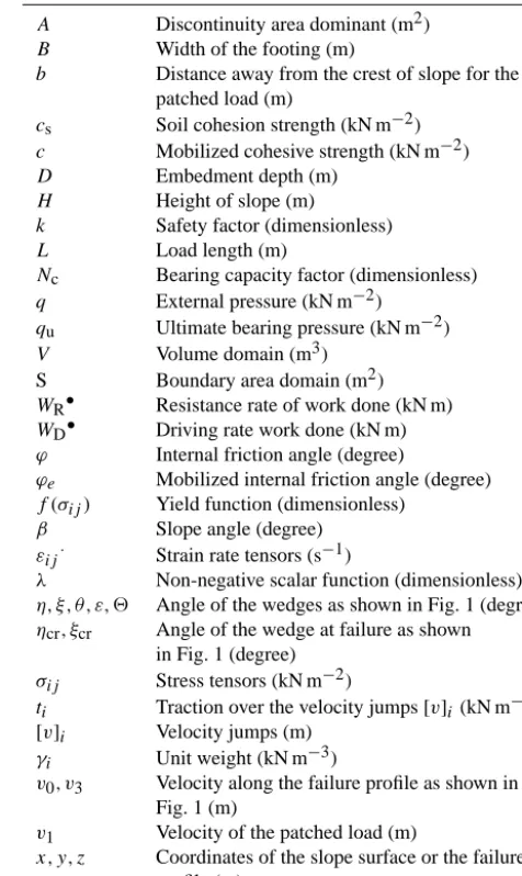
Table A1. Notation.
A Discontinuity area dominant (m2) B Width of the footing (m)
b Distance away from the crest of slope for the patched load (m)
cs Soil cohesion strength (kN m−2) c Mobilized cohesive strength (kN m−2)
D Embedment depth (m)
H Height of slope (m)
k Safety factor (dimensionless)
L Load length (m)
Nc Bearing capacity factor (dimensionless) q External pressure (kN m−2)
qu Ultimate bearing pressure (kN m−2)
V Volume domain (m3)
S Boundary area domain (m2) WR• Resistance rate of work done (kN m) WD• Driving rate work done (kN m) ϕ Internal friction angle (degree)
ϕe Mobilized internal friction angle (degree) f (σij) Yield function (dimensionless)
β Slope angle (degree)
εij· Strain rate tensors (s−1)
λ Non-negative scalar function (dimensionless) η, ξ, θ, ε, 2 Angle of the wedges as shown in Fig. 1 (degree) ηcr, ξcr Angle of the wedge at failure as shown
in Fig. 1 (degree) σij Stress tensors (kN m−2)
ti Traction over the velocity jumps[v]i(kN m−2) [v]i Velocity jumps (m)
γi Unit weight (kN m−3)
v0, v3 Velocity along the failure profile as shown in Fig. 1 (m)
v1 Velocity of the patched load (m)
Acknowledgements. The authors would like to thanks to the
support from The Hong Kong Polytechnic University through the account ZVCR and Research Grant Council project PolyU 5128/13E.
Edited by: T. Glade
Reviewed by: C. Zangerl and one anonymous referee
References
Azzouz, A. S. and Baligh, M. M.: Loaded areas on cohesive slopes, J. Geotech. Eng.-ASCE, 109, 709–729, 1983.
Bagge, G.:Tension cracks in saturated clay cutting, Proc. 11. th. Int. Conf. on. Soil Mechanics and Foundation Engineering, San Fran-cisco, 393–395, 12–16 August, 1985.
Baker, R.: Tensile strength, tensile cracks, and stability of slopes, Soils Found., 21, 1–17, 1981.
Bishop, A. W.: The use of the slip circle in stability analysis of slopes, Geotechnique, 5, 7–17, 1955.
Chen, J., Yin, J. H., and Lee, C. F.: Upper bound limit analysis of slope stability using rigid elements and nonlinear programming, Can. Geotech. J., 40, 742–752, 2003.
Chen, R. H. and Chameau, J. L.: Three dimensional limit equilib-rium analysis of slopes, Geotechnique, 32, 31–40, 1982. Chen, W. F.: Limit analysis and soil plasticity, 47–106, Elsevier
Sci-entific Publishing Company, USA, 1975.
Chen, W. F. and Liu, X. L.: Limit analysis in soil mechanics, 46 and 437–469, Elsevier Scientific Publishing Company, USA, 1990. Chen, Z., Wang, X., Haberfield, C., Yin, J. H., and Wang, Y.: A
three dimensional slope stability analysis method using the upper bound theorem, Part 1: Theory and methods, Int. J. Rock Mech. Min., 38, 369–378, 2001a.
Chen, Z., Wang, J., Wang, Y., Yin, J. H., and Haberfield, C.: A three dimensional slope stability analysis method using the upper bound theorem, Part 2: Numerical approaches, applications and extensions, Int. J. Rock Mech. Min., 38, 379–397, 2001b. Cheng, Y. M. and Au, S. K.: Slip line solution of bearing capacity
problems with inclined ground, Can. Geotech. J., 42, 1232–1241, 2005.
Cheng, Y. M. and Lau, C. K.: Slope Stability Analysis and Stabiliza-tion: New Methods and Insight, 2nd Edn., 54, CRC Press, Taylor & Fracis Group, USA, 2013.
Cheng, Y. M. and Yip, C. J.: “Three-dimensional Asymmetrical Slope Stability Analysis – Extension of Bishop’s and Janbu’s Techniques”, J. Geotech. Geoenviron., 133, 1544–1555, 2007. Cheng, Y. M., Lansivarra, T., and Wei, W. B.: Two-dimensional
Slope Stability Analysis by Limit Equilibrium and Strength Re-duction Methods, Comput. Geotech., 34, 137–150, 2007.
Cheng, Y. M., Lansivaara, T., Baker, R., and Li, N.: The use of inter-nal and exterinter-nal variables and extremum principle in limit equi-librium formulations with application to bearing capacity and slope stability problems, Soils Found., 53, 130–143, 2013a. Cheng, Y. M., Au, S. K., Pearson, A. M., and Li, N.: An innovative
Geonail System for soft ground stabilization, Soils Found., 53, 282–298, 2013b.
Farzaneh, O. and Askari, F.: Three-dimensional analysis of nonho-mogeneous slopes, J. Geotech. Geoenviron.-Eng., 129, 137–145, 2003.
Giger, M. W. and Krizek, R. J.: Stability analysis of vertical cut with variable corner angle, Soils Found., 15, 63–71, 1975.
Hovland, H. J.: Three dimensional slope stability analysis method, J. Geotech. Eng.-ASCE, 103, 971–986, 1977.
Hungr, O.: An extension of Bishop’s simplified method of slope stability analysis to three dimensions, Geotechnique, 37, 113– 117, 1987.
Huang, C. C. and Tsai, C. C.: New method for 3D and asymmetrical slope stability analysis, J. Geotech. Geoenviron., 126, 917–927, 2000.
Huang, C. C. and Tsai, C. C.: General method for three-dimensional slope stability analysis, J. Geotech. Geoenviron., 128, 836–848, 2002.
Janbu, N.: Slope stability computations, in: Embankment–Dam En-gineering, edited by: Hirschfield, R. C. and Poulos, S. J., John Wiley, 47–86, 1973.
Lam, L. and Fredlund, D. G.: A general limit equilibrium model for three-dimensional slope stability analysis, Can. Geotech. J., 30, 905–919, 1993.
Li, N. and Cheng, Y. M.: Laboratory and 3-D distinct element anal-ysis of the failure mechanism of a slope under external surcharge, Nat. Hazards Earth Syst. Sci., 15, 35–43, doi:10.5194/nhess-15-35-2015, 2015.
Michalowski, R. L.: Three dimensional analysis of locally loaded slopes. Geotechnique, 39, 27–38, 1989.
Morgenstern, N. R. and Price, V. E.: The analysis of stability of general slip surfaces, Geotechnique, 15, 79–93, 1965.
Prandtl, L.: Über die Härte Plastischer Körper. Göttingen Nachr., Mathematisch Physikalische Klasse, 12, 74–85, 1920.
Sokolovskii, V. V.: Statics of Soil Media (translated by D. H. Jones and A. N. Scholfield), Butterworths Scientific, London, 1960. Spencer, E.: A method of analysis of the stability of embankments
assuming parallel inter-slice forces, Geotechnique, 17, 11–26, 1967.