Face Recognition using SIFT by varying Distance
Calculation Matching Method
Hirdesh Kumar
PEC University of Technology Sector-12,
Chandigarh (India)
Padmavati
PEC University of Technology Sector-12,
Chandigarh (India)
ABSTRACT
Scale Invariant Feature Transform (SIFT) is a method for extracting distinctive invariant feature from images [1]. SIFT has been applied to many problems such as face recognition and object recognition [18], [19], [20], [21]. We have analyzed performance of SIFT using Euclidean distance as a matching algorithm. Further the matching rate can be enhanced/improved by changing distance calculation methods used for matching between two face images. So this paper also describes face recognition under various distance calculation methods like Correlation and Cosine. The experiments are conducted on different images of ORL face database [17] and Indian Face database [16] by changing illumination condition, scaling and rotation. From the experiments, it is shown that cosine and correlation distance calculation methods have performed well compared to the Euclidean distance matching method of original SIFT.
General Terms
Face Recognition, Object Recognition, Image Matching, Recognition.
Keywords
Face recognition, Scale Invariant Feature Transform, SIFT.
1.
INTRODUCTION
Feature extraction is a basic need under image processing field, because face recognition, object recognition, robot navigation, object detection etc needs feature for matching purpose. Image matching is considered as a solution of various problems such as object tracking, object recognition, three dimension reconstructions, etc. There are number of feature extraction techniques available [2], [5], [6], [7]. We use SIFT (Scale Invariant Feature Transformation), because it is one of the most robust technique for feature extraction [11]. The SIFT descriptor can transform image information into scale invariant feature keypoints. The SIFT descriptor remain invariant under rotation, scaling, and variation in lightning condition. In original SIFT algorithm Euclidian distance is used for matching keypoints.
2.
THE SIFT ALGORITHM
Here, we present overview of SIFT keypoint descriptor. The SIFT algorithm transforms image data into scale invariant feature. The four major steps of SIFT algorithm are as follows:
2.1
Scale-space extrema detection
In this step of SIFT candidate keypoints are detected, In this step first image is convolved with Gaussian filters at different
scales, and then we take the difference of successive Gaussian-blurred images [2].
A DoG image of image at different scale is given as:
)
,
,
(
)
,
,
(
)
,
,
(
x
y
L
x
y
k
iL
x
y
k
jD
Where L(x,y,k)is the convolution of the original image
)
,
(
x
y
I
with the Gaussian blurring G(x,y,k)at scale k i.e.
)
,
(
)
,
,
(
)
,
,
(
x
y
k
G
x
y
k
I
x
y
L
For scale space extrema detection in the SIFT algorithm, the convolved images are grouped by octave [3]. And we select the value of ki in such a manner that we obtain a fixed number of convolved images per octave. After this the DoG are taken from adjacent Gaussian-blurred images per octave.
After DoG images have been obtained, we have to identify local minima/maxima of the DoG images across scales. For this we have to compare each pixel in the DoG images to its eight neighbors at the same scale and nine corresponding neighboring pixels in each of the neighboring scales. If the pixel is maximum or minimum among all compared pixels, then this pixel is selected as a candidate key point.
2.2
Keypoint localization
After first step of SIFT too many candidate keypoints are produced, some of which are unstable. The keypoint localization step is used for discarding those points that have low contrast or poorly localized along an edge. This step has following three sub steps:
2.2.1
Interpolation of nearby data for accurate
position
This substep calculates the interpolated location of the extremum, which substantially improves matching and stability [1]. The quadratic Taylor expansion of the Difference-of-Gaussian scale-space function
D
(
x
,
y
,
)
, with the candidate keypoint as the origin is used for interpolation [1]. This Taylor expansion is given as:
x
x
D
x
x
Dx
D
D
x
D
TT
2 2
2
1
zero. If the X is larger than 0.5 in any dimension, then this means that the extremum close to other candidate keypoint. So the candidate keypoint is changed and the interpolation performed instead about that point. Otherwise the offset is added to its candidate keypoint to get the interpolated location of the extremum.
2.2.2
Discarding low - contrast keypoints
In this substep we computed the value of D(x) at the offsetX . If this value is less than 0.03, the candidate
keypoint is discarded. Otherwise candidate keypoint is kept with final location Y+X and scale σ, where Y is the original
location of the keypoint.
2.2.3
Eliminating edge responses
The Difference of Gaussian will have strong responses along edges. So in order to increase stability, we need to eliminate those keypoints which have poorly determined locations but have high edge responses.
As we know principal curvature across the edge are larger than the principal curvature along the edges, for poorly defined peaks in the DoG function. Finding these principal curvatures equal to solving for the eigenvalues of the second-order Hessian matrix, H:
yy xy xy xxD
D
D
D
H
The eigenvalues obtained from this Hessian matrix are proportional to the principal curvatures of D. If we have two eigenvalues α and β, in which α is larger and β is smaller than the ratio of these two values,
r
, is sufficient for SIFT's purpose. The trace of HD
xx
D
yy gives us the sum of the two eigenvalues, while the determinant2
xy yy
xx
D
D
D
gives us the product. Theratio
(
)
2(
)
H
Det
H
Tr
R
can be shown to be equalto r 2 r
) 1
( , so we can say that R depends only on the ratio of α and β. R is minimum when the eigenvalues are equal to each other. It follows that, for some threshold eigenvalue ratio rth, if value of R is greater
than
th th
r
r
1
)
2(
for a candidate keypoint then that keypoint is poorly localized and hence rejected.2.3
Orientation assignment
The current step is the key step in achieving invariance to rotation because keypoint descriptor can be represented relative to this orientation and therefore achieves invariance to image rotation.
First, the Gaussian-smoothed imageL(x,y,)at the keypoint's scale σ is taken so that all computations are performed in a scale-invariant manner. For an image
) , (x y
L at scale σ, the gradient magnitude,
m
(
x
,
y
)
, and orientation,
(
x
,
y
)
are computed as:2 2
))
1
,
(
)
1
,
(
(
))
,1
(
)
,1
(
(
)
,
(
x
y
L
x
y
L
x
y
L
x
y
L
x
y
m
)
,
1
(
)
,
1
(
)
1
,
(
)
1
,
(
tan
)
,
(
1y
x
L
y
x
L
y
x
L
y
x
L
y
x
The magnitude and direction calculations are done for every pixel in a neighboring region around the keypoint in the Gaussian-blurred image L. Each sample in the neighboring window added to a histogram bin. Once the histogram is filled, the orientations corresponding to the highest peak and local peaks that are within 80% of the highest peaks are assigned to the keypoint. If multiple orientations being assigned, an extra keypoint is created having the same location and scale as the original keypoint for each additional orientation.
2.4
Keypoint descriptor
This final step computes a descriptor vector for each keypoint such that the descriptor is highly distinctive and partially invariant to other variations such as illumination, 3D viewpoint, etc.
Initially a set of orientation histograms are created on 4x4 pixel neighborhoods with 8 bins each. Each histogram contains samples from a 4 x 4 sub-region of the original neighborhood region. The magnitudes are further weighted by a Gaussian function with σ =1.5 the width of the descriptor window. The descriptor then becomes a vector of all the values of these histograms. Since there are 4 x 4 = 16 histograms each with 8 bins, so the vector has 128 elements. In order to enhance invariance to affine changes in illumination, the vector is normalized to unit length.
3.
DISTANCE METHODS USED FOR
MATCHING
We used the following distance calculation method for matching between two face images:
3.1.1
Euclidean distance
Euclidean distance is the most popular and basic method for calculating the distance between two points or two vectors [14], [15]. This is the method used for matching in original SIFT algorithm. The Euclidean distance between vectors xs
and yt is given by:
'
)
)(
(
s t s tst
x
y
x
y
d
3.1.2
Cosine distance
Cosine distance between two vectors is calculated by measuring the cosine of angle between them [12], [15]. The cosine of 0 is 1 and less than 1 for other values. This is one of the most popular methods to calculate similarity between two documents. The cosine distance between two vectors is given by:
)
)(
(
1
' ' ' t t s s t s sty
y
x
x
y
x
d
Where xs and yt are the vectors.
3.1.3
Correlation distance
' '
'
)
)(
(
)
)(
(
)
)(
(
1
t t t t s s s s
t t s s st
y
y
y
y
x
x
x
x
y
y
x
x
d
Where
jsj
s
x
n
x
1
And
jtj
t
y
n
y
1
4.
EXPERIMENTS AND RESULTS
In 2006 Mohamad Aly apply SIFT on face image using cosine and angle matching methods [18]. For this paper we have we have conducted experiments on ORL face database and Indian face database. The ORL face database contains gray scale images while Indian face database contains color images. We have done for scaling, rotation, and illumination change (change in brightness and contrast). We have done matching using original David Lowe’s SIFT method and by cosine and correlation distance calculation matching method.
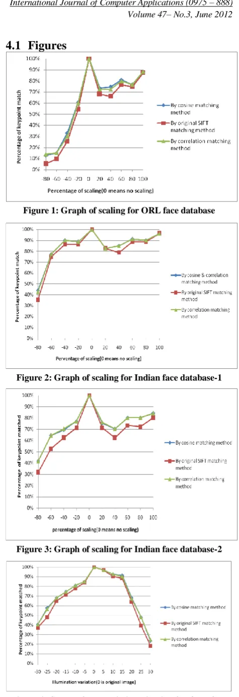
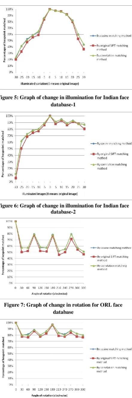
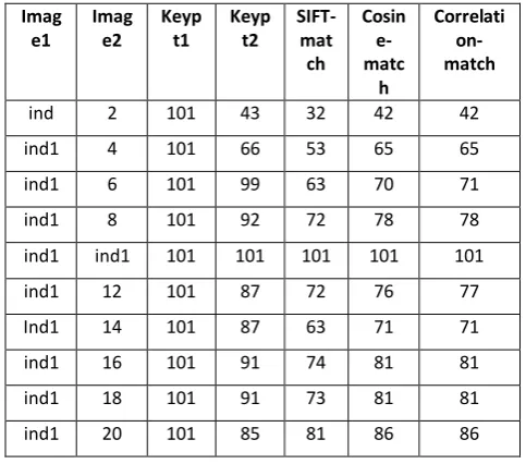
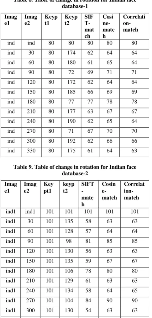
Figures 1-3 show the graphs for scaling and tables 1-3 show the tables for scaling. In figures 1-3, horizontal axis shows the angle of scaling while vertical axis shows percentage of keypoint matched. At horizontal axis 0 means no scaling, negative scaling shows the percentage of decrement and positive scaling shows percentage of increment in image size. Figure 1 shows scaling graph for ORL face database while table 1 shows scaling table for ORL face database. Figures 3 show scaling graphs for Indian face database while tables 2-3 show scaling tables for Indian face database. Figures 1-2-3 and tables 1-3 show that matching rate is enhanced for scaling by cosine and correlation matching methods as compare to original SIFT matching method (Euclidean distance method). Figures 4-6 show the graphs for illumination (Brightness and contrast) change and tables 4-6 show the tables for illumination change. In figures 4-6 horizontal axis shows change in illumination, while vertical axis shows percentage of keypoint matched. For illumination we take the scale from -100 to 100. Where at a change of -100 in illuminations whole image become black, while at a change of 100 in illuminations whole image become white. Change of 0 in illumination shows that the image is original. Figure 4 is illumination graph for ORL face database while table 4 is illumination table for ORL face database. Figures 5-6 are illumination graphs for Indian face database and tables 5-6 are illumination tables for Indian face database. From graphs and tables for illumination changes it is clear cosine and correlation matching methods give enhanced matching rate in case of illuminations change as compare to original SIFT. Figures 7-9 show the graphs for variation in rotation and tables 7-9 show the tables for variation in rotation. Here we consider rotation in clockwise direction. Here figure 7 and table 7 are rotation variation graph and table respectively for ORL face database while figures 8-9 and tables 8-9 are graphs and tables respectively for Indian face database. Here also cosine and correlation matching methods enhance the matching rate as compare to SIFT’s traditional matching method (Euclidean distance matching method) for rotation.
[image:3.595.310.548.39.733.2]4.1
Figures
Figure 1: Graph of scaling for ORL face database
Figure 2: Graph of scaling for Indian face database-1
Figure 3: Graph of scaling for Indian face database-2
[image:3.595.54.289.75.222.2]Figure 5: Graph of change in illumination for Indian face database-1
Figure 6: Graph of change in illumination for Indian face database-2
Figure 7: Graph of change in rotation for ORL face database
[image:4.595.314.549.75.216.2]Figure 8: Graph of change in rotation for Indian face database-1
Figure 9: Graph of change in rotation for Indian face database-2
4.2
Tables
Table 1. Table of scaling for ORL face database
Imag e1
Imag e2
keyp t1
keyp t2
matc h-SIFT
matc h-cosin
e
match-correlati
on
r10 2 94 6 5 12 13
r10 4 94 16 9 14 14
r10 6 94 33 24 31 29
r10 8 94 78 51 57 57
r10 r10 94 94 94 94 94
r10 12 94 118 64 69 68
r10 14 94 144 62 70 68
r10 16 94 222 72 76 75
r10 18 94 256 70 72 72
r10 20 94 277 82 83 83
Table 2. Table of scaling for Indian face database-1
Imag e1
Imag e2
keyp t1
keyp t2
SIFT-matc h
cosine -match
correlati on-match
ind 2 80 45 28 35 34
Ind 4 80 73 60 62 62
Ind 6 80 81 69 72 72
Ind 8 80 77 69 71 71
Ind Ind 80 80 80 80 80
Ind 12 80 75 66 66 66
Ind 14 80 73 63 68 68
Ind 16 80 84 71 73 73
Ind 18 80 74 71 72 72
[image:4.595.54.290.75.216.2]Table 3. Table of scaling for Indian face database-2
Imag e1
Imag e2
Keyp t1
Keyp t2
SIFT-mat ch
Cosin e-matc
h
Correlati on-match
ind 2 101 43 32 42 42
ind1 4 101 66 53 65 65
ind1 6 101 99 63 70 71
ind1 8 101 92 72 78 78
ind1 ind1 101 101 101 101 101
ind1 12 101 87 72 76 77
Ind1 14 101 87 63 71 71
ind1 16 101 91 74 81 81
ind1 18 101 91 73 81 81
ind1 20 101 85 81 86 86
Table 4. Table of change in illumination for ORL face database
Imag e1
Imag e2
Keyp t1
keyp t2
SIF T-mat
ch Cosi
ne-matc
h
Correlati on-match
r10 (-30) 94 62 35 38 38
r10 (-25) 94 69 45 54 53
r10 (-20) 94 72 61 64 64
r10 (-15) 94 83 67 70 70
r10 (-10) 94 83 73 76 76
r10 (-5) 94 88 79 80 80
r10 r10 94 94 94 94 94
r10 5 94 99 91 91 91
r10 10 94 105 85 87 87
r10 15 94 103 83 86 85
r10 20 94 86 60 64 63
r10 25 94 73 37 45 45
r10 30 94 57 17 22 23
Table 5. Table of change in illumination for Indian face database-1
Imag e1
Imag e2
Keyp t1
Keyp t2
SIF T-mat ch
Cosi ne-matc h
Correlati on-match
ind (-30) 80 32 16 18 19
Ind (-25) 80 28 26 33 33
Ind (-20) 80 45 38 42 41
Ind (-15) 80 51 44 47 47
Ind (-10) 80 54 47 51 52
Ind (-5) 80 74 67 69 69
Ind Ind 80 80 80 80 80
Ind 5 80 85 78 78 78
Ind 10 80 96 77 77 77
Ind 15 80 106 73 73 73
Ind 20 80 98 64 66 66
Ind 25 80 106 42 48 48
Ind 30 80 116 29 35 35
Table 6. Table of change in illumination for Indian face database-2
Imag e1
Imag e2
Keyp t1
Keyp t2
SIF T-mat ch
Cosin e-matc h
Correlati on-match
ind1 (-30) 101 39 5 12 12
ind1 (-25) 101 69 51 62 63
ind1 (-20) 101 78 69 73 73
ind1 (-15) 101 84 75 79 79
ind1 (-10) 101 86 78 81 81
ind1 (-5) 101 92 87 90 90
ind1 ind1 101 101 101 101 101
ind1 5 101 104 89 92 92
ind1 10 101 109 94 96 96
ind1 15 101 105 87 90 90
ind1 20 101 108 92 94 94
ind1 25 101 112 89 89 89
[image:5.595.46.288.92.305.2]ind1 30 101 111 81 88 88
Table 7. Table of change in rotation for ORL face database
Imag e1
Imag e2
Keyp t1
Keyp t2
SIF T-mat ch
Cosi ne-matc h
Correlati on-match
r10 r10 94 94 94 94 94
r10 30 94 117 47 54 54
r10 60 94 111 49 54 54
r10 90 94 79 73 75 75
r10 120 94 118 49 54 55
r10 150 94 125 48 54 54
r10 180 94 87 72 74 74
r10 210 94 112 43 49 49
r10 240 94 109 47 52 52
r10 270 94 88 72 75 75
r10 300 94 107 51 54 54
[image:5.595.306.550.182.718.2]Table 8. Table of change in rotation for Indian face database-1
Imag e1
Imag e2
Keyp t1
Keyp t2
SIF T-mat ch
Cosi ne-matc h
Correlati on-match
ind ind 80 80 80 80 80
ind 30 80 174 62 64 64
ind 60 80 180 61 65 64
ind 90 80 72 69 71 71
ind 120 80 172 62 64 64
ind 150 80 185 66 69 69
ind 180 80 77 77 78 78
ind 210 80 177 63 67 67
ind 240 80 190 62 65 64
ind 270 80 71 67 70 70
ind 300 80 192 62 66 66
ind 330 80 175 61 64 63
Table 9. Table of change in rotation for Indian face database-2
Imag e1
Imag e2
Key pt1
keyp t2
SIFT -matc h
Cosin e-match
Correlat ion-match
ind1 ind1 101 101 101 101 101
ind1 30 101 135 58 63 63
ind1 60 101 128 57 64 64
ind1 90 101 98 81 85 85
ind1 120 101 130 56 63 63
ind1 150 101 135 59 67 67
ind1 180 101 106 78 80 80
ind1 210 101 129 61 63 63
ind1 240 101 134 58 64 65
ind1 270 101 104 84 90 90
ind1 300 101 130 54 63 63
ind1 330 101 127 60 65 66
5.
CONCLUSION AND FUTURE SCOPE
In this paper SIFT matching algorithm is analyzed. In this paper we used cosine and correlation distance calculation methods for matching and compare the results with Euclidean distance matching method’s result. We have done comparison based on three parameters that are scaling, illumination changes and rotation. The result shows that using cosine and correlation matching methods, matching rate is enhanced as compared to Euclidean distance matching method of original SIFT.
Here we provide some direction for future research that can be attempted:
We can further improve the matching rate by developing matching methods which are robust in comparison to methods we used.
We can improve the matching rate of those algorithm which uses SIFT as a part i.e. PCA-SIFT (Principal component analysis SIFT).
6.
REFERENCES
[1] Lowe, D. 2004 “Distinctive image features from scale-invariant keypoints”, International Journal of Computer Vision, Vol.60, no.2, 91–110.
[2] Mikolajczyk, K. and Schmid, C. 2002 “An affine invariant interest point detector”, In European Conference on Computer Vision,(ECCV), Copenhagen, Denmark, 128–142.
[3] Lindeberg, T. 1994 “Scale-space theory: A basic tool for analyzing structures at different scales”, Journal of Applied Statistics, vol.21, no.2, 224–270.
[4] Beis, J. and Lowe, D. 1997 “Shape indexing using approximate nearest-neighbor search in high-dimensional spaces”, In Proceedings of the International Conference on Computer Vision and Pattern Recognition, 1000– 1006.
[5] Brown, M. and Lowe, D. 2002 “Invariant Features from Interest Point Groups”, In Proceedings of the 13th British Machine Vision Conference, Cardiff, 253–262.
[6] Lowe, D. 1999 “Object Recognition from Local Scale Invariant Features”, In Proceedings of the International Conference on Computer Vision, Corfu, Greece, 1150– 1157.
[7] Schmid, C. and Mohr, R. 1997 “Local Gray value Invariants for Image Retrieval”, IEEE Transactions on Pattern Analysis and Machine Intelligence, 530–535. [8] Mikolajczyk, K. and Schmid, C. 2005 “A performance
evaluation of local descriptors”, IEEE Transactions on Pattern Analysis and Machine Intelligence, 1615–1630. [9] Fergus, R., Perona, P. and Zisserman, A. 2003 “Object
class recognition by unsupervised scale-invariant learning”, In IEEE Conference on Computer Vision and Pattern Recognition, Madison, Wisconsin, 264–271. [10]Lowe, D. 2001 “Local feature view clustering for 3D
object recognition”, IEEE Conference on Computer Vision and Pattern Recognition, Kauai, Hawaii, 682– 688.
[11]Ledwich, L. and Williams, S. “Reduced SIFT Features For Image Retrieval and Indoor Localisation”, Australasian Conf. on Robotics and Automation ACRA, Canberra.
[12]Strehl, A., Ghosh, J. and Mooney, R. 2000 “Impact of similarity measures on web-page clustering”, In AAAI-2000: Workshop on Artificial Intelligence for Web Search.
[13]Salton, G. 1989 “Automatic Text Processing”, Addison-Wesley, New York.
[14]Huang, A. 2008 “Similarity Measures for Text Document Clustering”, NZCSRSC 2008.
[image:6.595.47.290.83.591.2]http://www.mathworks.com/help/toolbox/stats/pdist2.ht ml.
Jain, V. and Mukherjee, A. 2002 “The Indian Face
Database”
http://vis-www.cs.umass.edu/~vidit/IndianFaceDatabase/
[16]The ORL face database is available for download on the Internet through Olivetti Research Limited’s web server at:
http://www.cl.cam.ac.uk/research/dtg/attarchive/pub/data /att_faces.zip
[17]Aly, M. 2006 “Face recognition using sift features”, CNS186 Term Project Winter 2006.
[18]Krizaj, J., Struc, V. and Pavesic, N. M. 2010 “Adaptation of SIFT features for face recognition under varying illumination”, Proceedings of the 33rd International Convention, pp. 691-694.
[19]Majumdar, A. and Ward, R. K., 2009 “Discriminative SIFT features for face recognition”, Canadian Conference on Digital Object Identifier, pp. 27-30. [20]Wang, H., Yang, K., Gao, F. and Li, J. 2011