https://doi.org/10.5194/nhess-17-993-2017 © Author(s) 2017. This work is distributed under the Creative Commons Attribution 3.0 License.
Simple and approximate estimations of future precipitation
return values
Rasmus E. Benestad, Kajsa M. Parding, Abdelkader Mezghani, and Anita V. Dyrrdal
The Norwegian Meteorological Institute, Henrik Mohns Plass 1, Oslo, 0313, Norway Correspondence to:Rasmus E. Benestad ([email protected])
Received: 24 June 2016 – Discussion started: 26 July 2016
Revised: 5 April 2017 – Accepted: 28 May 2017 – Published: 3 July 2017
Abstract.We present estimates of future 20-year return
val-ues for 24 h precipitation based on multi-model ensembles of temperature projections and a crude method to quantify how warmer conditions may influence precipitation intensity. Our results suggest an increase by as much as 40–50 % pro-jected for 2100 for a number of locations in Europe, assum-ing the high Representative Concentration Pathway (RCP) 8.5 emission scenario. The new strategy was based on com-bining physical understandings with the limited information available, and it utilised the covariance between the mean seasonal variations in precipitation intensity and the North Atlantic saturation vapour pressure. Rather than estimating the expected values and interannual variability, we tried to estimate an “upper bound” for the response in the precip-itation intensity based on the assumption that the seasonal variations in the precipitation intensity are caused by the seasonal variations in temperature. Return values were sub-sequently derived from the estimated precipitation intensity through a simple and approximate scheme that combined the 1-year 24 h precipitation return values and downscaled an-nual wet-day mean precipitation for a 20-year event. The lat-ter was based on the 95th percentile of a multi-model ensem-ble spread of downscaled climate model results. We found geographical variations in the shape of the seasonal cycle of the wet-day mean precipitation which suggest that different rain-producing mechanisms dominate in different regions. These differences indicate that the simple method used here to estimate the response of precipitation intensity to temper-ature was more appropriate for convective precipitation than for orographic rainfall.
1 Introduction
regional climate models (RCMs), which also have a mini-mum skillful scale (Takayabu et al., 2015) and have a lim-ited ability to reproduce the observed precipitation statistics (Orskaug et al., 2011; Benestad and Haugen, 2007). Nev-ertheless, RCMs have been used to study precipitation ex-tremes (e.g. Frei et al., 2006), although the heavy compu-tational demands have limited analysis to a small number of GCMs which means that the ensembles do not provide a real-istic range of possible outcomes associated with natural vari-ability and model uncertainty (Deser et al., 2012).
Traditional methods of estimating return values that make use of extreme value theory (EVT) are sensitive to sampling fluctuations and require long data records to avoid extrap-olation of extreme characteristics (Coles, 2001; Papalexiou and Koutsoyiannis, 2013). Extreme precipitation modelled through EVT usually describes amounts that are far out in the tail of the distribution and associated with low probability, and the estimates may change when new extremes are sam-pled. Most uses of EVT also assume stationarity, although there are ways to account for trends (Cheng et al., 2014).
Local precipitation has been notoriously difficult to predict (Stocker et al., 2013; Field et al., 2012; Arkin et al., 1994); one reason may be that it has involved quantities such as the monthly mean precipitation that are calculated from a blend of different (both dry- and wet-day) conditions and phenom-ena without accounting for these differences. There are many different types of phenomena that generate precipitation, e.g. the formation of nimbostratus, mid-latitude cyclones, fronts, atmospheric rivers, convection and warm and cold initiation of rain (Fleagle and Businger, 1980; Berg et al., 2013; Tren-berth et al., 2003). Some of these have a stronger presence in certain regions and seasons. For instance, convective precip-itation is typically a summer phenomenon at mid-to-high lat-itudes, whereas mid-latitude cyclones are more pronounced in autumn, winter and spring. Another reason for the limited success may be the small sample size in calculations of the mean precipitation for locations and seasons where it rains rarely. For example, if it rains less than 30 % of the total number of days in a month, the monthly average precipita-tion is based on less than 10 values. The quantificaprecipita-tion of future extreme precipitation is associated with uncertainties from a number of sources (e.g. model imperfections, spar-sity of data, sensitivity to random variations in small samples constituting the tail of the distribution, non-stationarity and the representation of natural variability). Large multi-model ensembles can be used to explore the natural variability of the climate system, although the range of the ensembles also in-cludes other sources of uncertainty and variability, and some ensemble members may be inter-dependent (Sanderson et al., 2015).
Moderate extremes in 24 h precipitation amounts (X) can be approximated with an exponential distribution (Benestad et al., 2012a, b; Benestad, 2013), which is described with one parameter – the wet-day meanµ– and its percentile (qp) can
be estimated as qp= −ln(1−p)µ. The exponential
distri-● ●
●
●
●
● ●●
●
●
●
●
2600 2800 3000 3200 3400
3
4
5
6
7
"Worst−case" fit based on seasonal variations
es (Pa) VELIKIE LUKI (30.62° E/56.35° N; 97ma.s.l.)
µ
(mm
day
-1)
● ●
●
●
●
● ●●
●
●
●
●
Correlation = 0.97 ( p−value = 0 %) Regression: y = −7.2397 + 0.0041 x (R2 = 0.95 )
Jan Mar May Jul Sep Nov
Figure 1.A comparison between the mean seasonal cycle in the
saturation vapour pressure (xaxis) and the wet-day mean (yaxis)
for the site Velikie Luki, Russia. The error bars indicate 2 standard deviations of the year-to-year variations in the two variables. An inset shows the standardised seasonal cycles, both variables peaking
in July–August (red line=es, blue line=µ).
bution can be used to estimate changes in the moderate up-per tail of the statistical distribution, assuming that these fol-low changes in the bulk characteristics where the probability adds up to unity (Benestad and Mezghani, 2015). This ap-proximation has been tested against daily rain-gauge records from around the world, confirming that the exponential dis-tribution (qp= −ln(1−p)µ) predicts the observed precipi-tation percentiles with high accuracy for low-to-moderately heavy precipitation amounts (Fig. S1 in the Supplement). This means thatµis useful for risk analysis to estimate upper percentiles of 24 h precipitation amounts because the 95th percentileq95 is expected to change proportionally with µ
(Benestad, 2013; Benestad and Mezghani, 2015).
2 Data and methods
sea-sonal variations, ensemble spread and different physical pro-cesses present during wet and dry days.
The estimated precipitation change was based on the change in temperature and did not explicitly take atmo-spheric circulation changes or feedback processes into con-sideration. This change can, for all intents and purposes, be interpreted as a zeroth-order measure of an “upper bound” of change in precipitation intensity associated with increased temperature, rather than the most likely value. Attributing all of the seasonal variations in the precipitation intensity to its covariance with temperature may inflate the role of the tem-perature, as other factors exhibit a similar mean seasonal cy-cle and may have an influence on the precipitation intensity. For this reason, we use the terms upper bound and potential sensitivity. It is also true that other unaccounted-for processes possibly may influence precipitation intensity in a nonlinear fashion and possibly result in even higher intensities if they also change in the future. However, as long as (a) such fac-tors have an approximately linear dependency on the tem-perature and (b) the temtem-perature may be taken as a proxy for climate change, then this simple assumption may provide a reasonable figure. This simple method differs from tradi-tional methods in that rather than attempting to specify the most likely value, it estimates a kind ofupper boundof the systematic response of extreme precipitation to changes in temperature. We henceforth describe this relation as the po-tential sensitivity (PS) since the calibration used the covari-ance of the mean annual variation that may exaggerate the effect of the temperature. This is described in more details below.
Our approach was based on empirical–statistical down-scaling (ESD) applied to a large multi-model ensemble to provide estimates of return values for heavy precipitation, and is an alternative to EVT-based approaches. It provided an estimate that was more approximate and crude, but less sensitive to outliers because a larger portion of the data sam-ple is used.
The Supplement provides more details and explanations of the strategy, as well as the R scripts used to perform the analysis. The calculations and graphics were produced with the open-source R package “esd” (Benestad et al., 2015). The data used in this analysis are available from the reference provided in Benestad (2017).
2.1 Data
Precipitation observations were obtained from the daily Eu-ropean Climate Assessment, ECA&D, data set (Klein Tank et al., 2002) for 1032 stations in northern Europe with data available for the time period 1961–2014 (Fig. 2). Surface temperature data from the National Centers for Environ-mental Prediction/National Center for Atmospheric Research (NCEP/NCAR) Reanalysis 1 (Kalnay et al., 1996) over a selected North Atlantic domain (100◦W–30◦E/0◦N–40◦N; see Fig. S2) were used to calculate the predictors for the
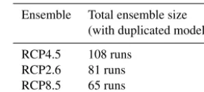
Table 1.Summary of the CMIP5 experiments. RCP4.5 was used as default here, whereas RCP2.6 and 8.5 were taken as lower and upper limits based on different emission scenarios.
Ensemble Total ensemble size
(with duplicated models)
RCP4.5 108 runs
RCP2.6 81 runs
RCP8.5 65 runs
downscaling, and corresponding projections from the CMIP5 ensembles of GCMs assuming the Representative Concen-tration Pathway (RCP) 2.6, 4.5 and 8.5 scenarios (Taylor et al., 2012) were used for the projections of future change (Ta-ble 1). We used the NCEP/NCAR Reanalysis 1 because the data covered the 1961–2014 period and because it provided a representation for the surface temperature that was compa-rable to that of the CMIP5 GCMs.
2.2 Downscaling method
2.2.1 Predictand: annual wet-day mean precipitation
A traditional approach for modelling and analysing precipi-tation typically involves the monthly mean precipiprecipi-tation (X), but in this study, we instead downscaled the wet-day mean,
µ. In this analysis we usedµto represent the wet-day mean precipitation in general, reflecting both the annual wet-day mean precipitation and the mean seasonal variations in the wet-day mean precipitation estimated for the 12 calendar months. The mean precipitation was not the optimal quantity for describing precipitation statistics because in most places it does not rain every day, and the proportion of wet days to total number of days in a monthly sample can have im-plications for the estimation of the statistical parameters de-scribing the distribution. The mean precipitation can be ex-pressed as the product of the wet-day frequency (fw) andµ
according toX=fwµ. A comparison between the seasonal dependence ofX,µand wet-day frequency fw indicated a stronger seasonal cycle inµthan infwandX(see Fig. S3). The weaker seasonal cycle inX was due to the blending of different types of weather conditions in the mean precipita-tion. The strong seasonal cycle ofµindicated a sensitivity to climatological variations, which is an important requirement for the statistical downscaling strategy proposed here.
2.2.2 Predictor: the saturation vapour pressure
We assumed that the vapour saturation pressure,es, is more
linearly related to the atmospheric water content and precip-itation than the temperature, and hence we usedesas a
esti- lon(x) lon(x)
(a)Annual cycle in PC 1 with variance of 54 %
−0.06 −0.04 −0.02 0.00 0.02 0.04 0.06 0.08 breaks −0.2 0.0 0.2 0.4 Index pca$u[, ipca]
Jan Apr Jun Sep Dec
lon(x) lon(x)
(b) Annual cycle in PC 2 with variance of 40 %
0.00 0.05 0.10 breaks −0.4 −0.2 0.0 0.2 0.4 Index pca$u[, ipca]
Jan Apr Jun Sep Dec
Figure 2b
Figure 2. The weights for the two leading principal
compo-nents (a, b)of the seasonal cycle of the wet-day mean
precipita-tionµin the 1032 rain gauge records. The colour of the symbols
indicates how strongly the shape is present in the local seasonal
cy-cle, and the size reflectsR2from the regression analysis between
es andµ(see Fig. S5). Filled circles were used for locations with
R2>0.6, hollow circles for 0.6≥R2>0.4 and crosses indicate
locations withR2<0.4. The shape of the seasonal cycle principal
component forµis shown in the inset (top left of each panel).
mated from the surface temperature (0.995σlevel),T.
es=10(11.40−2353/T ) (1)
This approximation was based on integration of the Clausius–Clapeyron equation, assuming a constant latent heat of vaporisation (see Eq. 2.89 in Fleagle and Businger, 1980). The mean seasonal variations in the regional aver-agees over the North Atlantic domain was used as
predic-tor forµ, based on its mean seasonal variation (Fig. 1); our reasoning was that it can be considered as the source region for humidity in Europe. The domain was set after some tri-als for a few test stations, but no systematic study or tuning of the predictor domain was conducted. The predictor index was calculated from gridded temperature data from reanaly-ses and global climate models (GCMs) and was then spatially and temporally aggregated where monthly griddedesvalues were estimated according to Eq. (1) and surface temperatures from the multi-model ensemble, and were used to downscale an ensemble of local results of annual wet-day mean precip-itationµˆ (hereµˆ is used for predicted annual mean).
2.2.3 The empirical–statistical model
A model for predicting the annual wet-day mean precipi-tation µˆ can be constructed as a sum of a constant, β0, a term depending on the saturation vapour pressure,βTes, and
a Gaussian noise term,N (0, σ ), assuming that factors other than temperature that are affecting wet-day precipitation are stochastic and stationary:
ˆ
µ=β0+βTes+N (0, σ ). (2)
The assumptions about other factors being stationary and stochastic is partly based on the heuristic notion of physical interdependencies between various aspects of the planetary atmosphere in general and that the temperature is a proxy for such influences. One example may be the cloud top height which is expected to be influenced by the convective avail-able potential energy (CAPE) that is sensitive to tempera-tures. We used the observed standard deviation ofµin the month with the highest interannual variability as an estimate of the standard deviationσof the noise termN, which in this case was August. We calculated the coefficientsβ0andβT
using linear regression analysis between the mean seasonal cycle of the observed monthly meanµand the correspond-ing seasonal cycle of the regionally averagedes calculated from reanalysis temperature data from the Atlantic domain, as described in Sect. 2.2.2. The coefficientβT is the scaling
ratio which we refer to as the potential sensitivity.
also exhibit a seasonal cycle and interfere with the regression analysis so that the coefficient is weaker or stronger than the true influence of temperature on precipitation.
A 90 % uncertainty range for µˆ was estimated for the projections based on the ensembles of downscaled results, taken as the limit between the 5th and 95th percentiles (see, e.g., Fig. S4). This interval included the noise termN (0, σ ), and captured the observed year-to-year variations as well as model differences (Deser et al., 2012). We assumed that the multi-model ensemble spread for any given year could approximately represent the typical year-to-year variance, which meant that the 95th percentile forµˆ, which we hence-forth refer to asµ95ˆ , could be used as a proxy for the value to be exceeded once in 20 years (Benestad, 2016) (the 20-year event has a probability of 0.05 (1/20) of occurring in a given year, and the 95th percentile represents a limit that only 5 % (1 in 20) of the distribution exceeds).
2.3 Return value probabilities
To estimate future return values based on the downscaled ˆ
µ, we again assumed that the wet-day precipitation amount was exponentially distributed and that the probability for 24 h precipitation exceeding a critical thresholdxcould be calcu-lated as follows:
Pr(X > x)≈fwe−x/µ, (3)
where fw was the wet-day frequency (Benestad and Mezghani, 2015). Previous analysis suggest that the expo-nential distribution gives a reasonable description of the probabilities for moderate precipitation events such as the 95-percentile, but is not expected to be suitable for rare extremes much beyond the 20-year return level (Benestad, 2013).
The probability associated with the 1-year return value of 24 h precipitation is approximately Pr(X > x)=1/365.25, and the corresponding threshold value was approximated ac-cording to
x1 year≈µ ln(365.25fw). (4)
Previous comparison between the return values based on Eq. (4) and general extreme value theory, has suggested that they give roughly similar results (Benestad and Mezghani, 2015). A test of Eq. (4) indicated that the return values scale withµ: values ofx1 year that were associated with high per-centiles and low values ofµˆ approximately corresponded to
x1 year with low percentiles and high values ofµˆ (Fig. S1).
Based on Eq. (4), we made a rough estimate of the 20-year return value for the 24 h precipitation amount (x20 year) by
replacingµwith the 20-year return value of the annual wet-day mean. The estimate forxˆ20 yearwas calculated based on
the downscaled annual wet-day mean precipitation, using the 95th percentileµˆ95as a proxy for the 20-year return values:
ˆ
x20 year= ˆµ95 ln(365.25fw). (5)
In calculating future return values, we neglected changes infwand simply assumed that it will remain constant. Pre-vious analysis has indicated that the wet-day frequency is strongly influenced by circulation patterns (Benestad and Mezghani, 2015), and that it is closely connected to slow nat-ural variations such as the North Atlantic Oscillation (NAO) (Hurrell, 1995). Such natural variations are difficult to pre-dict and there is little evidence of a systematic shift in the frequency of different circulation patterns.
2.4 Principle component analysis of the seasonal cycle
Principal component analysis (PCA) was used to extract the most dominant shapes of the seasonal cycle inµamongst the observation sites (Fig. 2). The mean seasonal cycle was esti-mated for each site and used to construct a data matrixXwith 12 columns (one for each month) andnrows (one for each site). Singular value decomposition (SVD) was then used to compute the principal components:U6VT =X, whereUis the left inverse,Vthe right inverse and6 is a diagonal ma-trix holding the eigenvalues (Press et al., 1989; Strang, 1988). The procedure deconstructed the data into a set of shapes of the seasonal cycle, corresponding eigenvalues that described the explained variance and a spatial matrix that described the relative strength of each shape at the different locations.
3 Results and discussion
3.1 Potential sensitivity and the seasonal cycles inµ
andes
The mean seasonal cycles ofµat many European locations co-varied with the mean seasonal cycle ofesin the North At-lantic domain. This can be seen as a validation of the assump-tions underlying the empirical model, because the downscal-ing models were based on the regression between the sea-sonal cycles ofes andµ (Eq. 2). Figure 1 provides an
ex-ample of a scatter plot between the mean seasonal variations ines (x axis) and the corresponding cycle inµ(y axis) for
one location (Velikie Luki, Russia). The example in Fig. 1 was not unique: there was a high and statistically significant correlation (R2>0.6; Fig. S5) between the seasonal cycle of these two quantities for many of the rain gauge records (612 of the 1032 stations). The majority of the locations with a poor fit (R2<0.6) were found along the western coast of Norway and south-east of the Alps, while inland sites and locations in central Europe had higherR2values (see Fig. 2 where the size of the markers is proportional toR2). This in-dicated that a linear relationship betweenµandescould not
be expected in regions where orographic precipitation was dominant. Downscaled projections were carried out only for the locations with a good fit (R2>0.6).
that factors other than temperature also played a role in pre-cipitation variations. The downscaling strategy adopted here was designed to evaluate the maximum potential effect of temperature changes on the wet-day mean precipitation, and the scaling factor between the two is described as the poten-tial sensitivity. Since other processes also influenced precip-itation, the method could not be expected to reproduce past interannual variability, but it could be used to obtain a rough estimate of the effect of temperature changes on precipita-tion.
Figure 2 presents maps showing the two major compo-nents of the mean seasonal cycle in µ, which together ac-counted for 94 % of the variability for the 1032 locations examined. The spatial patterns in the principle components (PC) revealed different seasonal cycles of precipitation along the mountainous western coast of Norway and close to the Alps compared to the rest of Europe, probably related to oro-graphic effects. There was a gradient in the shape of the mean seasonal cycle inµwith the distance from the coast that was particularly visible over the Netherlands. Inland sites indi-cated higher precipitation intensities during July and August, which could be associated with convective rainfall. We found a positive correlation between the spatial vector of the lead-ing PCs andR2of the seasonal cycles ofesandµ: 0.82 (with
a 90 % uncertainty range of 0.80, 0.84), but negative corre-lation for mode 2 (−0.84;−0.86,−0.82) and no significant correlation for mode 3 (0.00; −0.06, 0.06). This indicated that the dominant shapes of the seasonal cycle ofµ in Eu-rope were associated with a strong connection to the North Atlantic temperature.
3.2 Projections of future precipitation
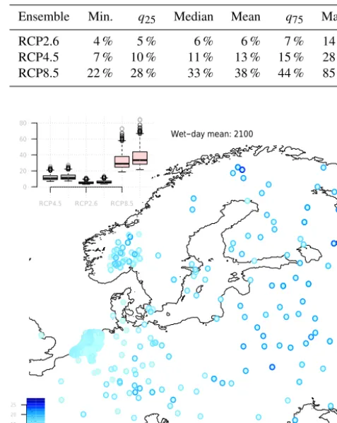
Projected values of the annual mean wet-day mean,µˆ, based on the downscaling model (Eq. 2) applied to the CMIP5 en-semble, are shown in Fig. 3. The downscaled results sug-gested an increase of up to 13 % in the wet-day mean from 2010 to 2100, assuming the RCP4.5 emission scenario (Stocker et al., 2013), and as much as 38 % at many of the lo-cations given the high emission scenario RCP8.5. The most extreme estimate was an 85 % increase at Sihccajavri (Nor-way). Since the wet-day precipitation amount approximately followed an exponential distribution, the proportional change in any percentile was the same as forµ. The inset in Fig. 3 shows estimated changes for the emission scenarios RCP4.5, 2.6 and 8.5 for both the ensemble mean and 95th percentile.
An analysis of historical observations provided some in-dication of skill of the downscaling models in terms of pre-dicting trends ofµbased on the North Atlantic temperature (Fig. S6). The historical trends exhibited a more pronounced scatter than the predicted trends, suggesting that factors other than the sea-surface temperature also had influenced the long-term changes. For most locations, there was an increase in µ between 1961 and 2014, typically 0.1 mm day−1 per decade (Fig. S6–S7).
Table 2.Summary of the projected change from 2010 to 2100 in the 20-year return value for 24 h precipitation under the assump-tion of staassump-tionary wet-day frequency. The sample comprises the 615 locations shown in Fig. 3. The numbers represent the change in per-centage with respect to year 2010.
Ensemble Min. q25 Median Mean q75 Max.
RCP2.6 4 % 5 % 6 % 6 % 7 % 14 %
RCP4.5 7 % 10 % 11 % 13 % 15 % 28 %
RCP8.5 22 % 28 % 33 % 38 % 44 % 85 %
● ● ● ● ● ● ● ● ● ● ● ● ● ● ● ● ● ● ● ● ● ● ● ● ● ● ● ●● ● ● ● ● ● ● ● ● ● ● ● ● ● ● ● ● ● ● ● ● ● ● ● ● ● ●● ● ● ● ● ● ● ● ● ● ● ● ● ● ● ● ● ● ● ● ● ● ● ●●●●●●●●●●●● ● ● ● ● ● ● ● ● ●● ● ●●● ● ● ● ● ● ● ●● ● ● ● ●● ● ● ● ●●● ● ●● ● ●● ●●● ● ● ●● ● ● ● ●● ● ● ● ● ● ● ● ● ● ● ● ● ● ●● ● ● ●●● ● ●● ● ● ● ● ● ● ●● ● ●● ● ● ● ● ● ●●●● ● ●●● ● ●● ● ● ●●● ●● ●● ●● ● ● ●●●●●● ● ● ●● ● ● ● ● ● ●●● ●● ● ●●●●●● ● ●● ●● ●● ● ●●●● ● ● ● ● ● ● ● ● ●● ● ● ● ● ● ●●●●● ● ● ● ● ● ● ● ● ● ● ● ● ●●● ● ● ● ●● ● ● ●● ●● ● ● ● ● ● ● ● ● ● ● ●●● ●●●●●● ● ● ●● ● ●●●● ● ● ● ●● ●●● ● ●● ● ● ● ● ●● ● ● ● ● ● ● ● ●● ● ● ● ●●●●● ● ● ● ● ● ● ● ●●● ● ● ●●● ● ● ● ● ●● ● ●● ● ● ● ● ● ●● ● ● ● ● ● ● ● ● ● ● ● ● ● ● ● ● ● ● ● ● ● ● ● ●● ●● ● ● ● ● ●●●●● ● ● ● ● ● ● ● ● ● ● ● ● ● ●●● ● ● ● ● ● ● ●●●●●●●●●●● ● ● ● ● ●●●●●●●●● ● ● ● ● ● ●●●●●●●● ●●●●●●● ● ● ● ●●● ● ● ● ● ● ● ●●●● ● ● ●●●●●●●●●● ●●●●●●●●●● ●●●●●●●●●● ●●●● ●● ●● ● ●● ● ● ● ● ● ● ● ● ● ● ● ● ● ● ● ● ● ● ● ● ● ● ● ● ● ● ● ● ● ● ● ● ● ● ● ● ● ● ● ● ● ● ● ● ●● ● ● ●● ● ● ● ● ● ● ● ● ● ● ● ● ● ● ● ● ●● ●● ● ● lon(x) lon(x) ● ● ● ● ● ● ● ● ● ● ● ● ● ● ● ● ● ● ● ● ● ● ● ● ● ● ● ●● ● ● ● ● ● ● ● ● ● ● ● ● ● ● ● ● ● ● ● ● ● ● ● ● ● ●● ● ● ● ● ● ● ● ● ● ● ● ● ● ● ● ● ● ● ● ● ● ● ●●●●●●●●●●●● ● ● ● ● ● ● ● ● ●● ● ●●● ● ● ● ● ● ● ●● ● ● ● ●● ● ● ● ●●● ● ●● ● ●● ●●● ● ● ●● ● ● ● ●● ● ● ●● ● ● ● ● ● ● ● ● ●●● ● ● ●●● ● ●● ● ● ● ● ● ● ●● ● ●● ● ● ● ● ● ●●●● ● ●●● ● ●● ● ● ●●● ●●●●●● ● ● ●●●●●● ● ● ●● ● ● ● ● ● ●●● ●● ● ●●● ●●● ● ●● ●● ●● ● ●●●● ● ● ● ● ● ● ● ● ●● ● ● ● ● ● ●●●●● ● ● ● ● ● ● ● ● ● ● ● ● ●●● ● ● ● ●● ●● ●● ●● ● ● ● ● ● ● ● ● ● ● ●●● ●●●●●● ● ● ●● ● ●●●● ● ● ● ●●●●● ● ●● ● ● ● ● ●● ● ● ● ● ● ● ● ●● ● ● ● ●●●●● ● ● ● ● ● ●● ●●● ●● ●●● ● ● ● ● ●● ● ●● ●● ● ● ● ●● ● ● ● ● ● ● ● ● ● ● ● ● ● ● ● ● ● ● ● ● ● ● ● ●● ●● ● ● ● ● ●●●●● ● ● ● ● ● ● ● ● ● ● ● ● ● ●●● ● ● ● ● ● ● ●●●●●●●●●●● ● ● ● ● ●●●●●●●●● ● ● ● ● ●●●●●●●●●●●●●●●● ● ● ● ●●● ● ● ● ● ● ● ●●●● ● ●●●●●●●●●●● ●●●●●●●●●●●●●●●●●●●● ●●●● ●● ●● ● ●● ● ● ●● ● ● ● ● ● ● ● ● ● ● ● ●● ● ● ● ● ● ● ● ● ● ● ● ● ● ● ● ● ● ● ● ● ● ● ● ● ● ● ● ●● ● ● ●● ● ● ● ● ● ● ● ● ● ● ● ● ● ● ● ● ●● ●● ● ● ● ● ● ● ● ● ● ● ● ● ● ● ● ● ● ● ● ● ● ● ● ● ● ● ● ● ● ●● ● ● ● ● ● ● ● ● ● ● ● ● ● ● ● ● ● ● ● ● ● ● ● ● ● ●● ● ● ● ● ● ● ● ● ● ● ● ● ● ● ● ● ● ● ● ● ● ● ●●●●●●●●●●●● ● ● ● ● ● ● ● ● ●● ● ●●● ● ● ● ● ● ● ●● ● ● ● ●● ● ● ● ●●● ● ●● ● ●● ●●● ● ● ●● ● ● ● ●● ● ● ● ● ● ● ● ● ● ● ● ● ● ●● ● ● ●●● ● ●● ● ● ● ● ● ● ●● ● ●● ● ● ● ● ● ●●●● ● ●●● ● ●● ● ● ●●● ●● ●● ●● ● ● ●●●●●● ● ● ●● ● ● ● ● ● ●●● ●● ● ●●●●●● ● ●● ●● ●● ● ●●●● ● ● ● ● ● ● ● ● ●● ● ● ● ● ● ●●●●● ● ● ● ● ● ● ● ● ● ● ● ● ●●● ● ● ● ●● ● ● ●● ●● ● ● ● ● ● ● ● ● ● ● ●●● ●●●●●● ● ● ●● ● ●●●● ● ● ● ●● ●●● ● ●● ● ● ● ● ●● ● ● ● ● ● ● ● ●● ● ● ● ●●●●● ● ● ● ● ● ● ● ●●● ● ● ●●● ● ● ● ● ●● ● ●● ● ● ● ● ● ●● ● ● ● ● ● ● ● ● ● ● ● ● ● ● ● ● ● ● ● ● ● ● ● ●● ●● ● ● ● ● ●●●●● ● ● ● ● ● ● ● ● ● ● ● ● ● ●●● ● ● ● ● ● ● ●●●●●●●●●●● ● ● ● ● ●●●●●●●●● ● ● ● ● ● ●●●●●●●● ●●●●●●● ● ● ● ●●● ● ● ● ● ● ● ●●●● ● ● ●●●●●●●●●● ●●●●●●●●●● ●●●●●●●●●● ●●●● ●● ●● ● ●● ● ● ● ● ● ● ● ● ● ● ● ● ● ● ● ● ● ● ● ● ● ● ● ● ● ● ● ● ● ● ● ● ● ● ● ● ● ● ● ● ● ● ● ● ●● ● ● ●● ● ● ● ● ● ● ● ● ● ● ● ● ● ● ● ● ●● ●● ● ●
Wet−day mean: 2100
10 15 20 25 ● ● ● ● ● ● ● ● ● ● ● ● ● ● ● ● ● ● ● ● ● ● ● ● ● ● ● ● ● ● ● ● ● ● ● ● ● ●●●●●●●●●●●●●●●●●●●●●●●●●●●●●●●●●●●●● ● ● ● ● ● ● ● ● ● ● ● ● ● ● ● ● ● ● ● ● ● ● ● ● ● ● ● ● ● ● ● ● ● ● ● ● ● ● ● ●●●●●●●●●●●●●●●●●●●●●●●●●●●●●●●●●●●●●●● ● ● ● ● ● ● ● ● ● ● ● ● ● ● ● ● ● ● ● ● ● ● ● ● ● ● ● ● ● ● ● ● ● ● ● ● ● ● ● ● ● ● ● ● ● ● ● ● ● ● ● ● ● ● ● ● ● ● ● ● ● ● ● ● ● ● ● ● ● ● ● ● ● ● ● ● ● ● ● ● ● ● ● ● 0 20 40 60 80
RCP4.5 RCP2.6 RCP8.5
Figure 3.Projected local change from 2010 to 2100 in the
ensem-ble mean and 95th percentile annual meanµfor the RCP4.5
emis-sion scenario. The colour of the inner part of the symbols indicates changes in the ensemble mean and the outer part the 95th percentile in terms of percentages since 2010. The inset shows a boxplot of
the projected change inµ, both for the ensemble mean (left) and
the 95th percentile (right) of emission scenarios RCP4.5, 2.6 and 8.5.
Estimates of future 20-year return values (Eq. 5) based onµ95ˆ and assuming a constant value of the wet-day fre-quency,fw, are shown in Table 2. Based on downscaling of the RCP4.5 scenario, the 20-year return values may increase by between 7 and 28 % by 2100 (ensemble median: 11 %), or assuming the high emission scenario RCP8.5, between 22 and 85 % (ensemble median: 33 %). Nevertheless, changes in
fwmay also influence return values, and an increase in the
number of rainy days would imply an even stronger change in return values.
The historical fw trends at the stations tend to cluster
1961–2014, but a less coherent pattern elsewhere (Fig. S9). This implied that factors other than the North Atlantic tem-perature may also have played a role in past trends and future precipitation changes. The wet-day frequency was strongly influenced by the circulation patterns (Benestad and Mezghani, 2015) and could potentially be predicted based on the mean sea-level pressure, but here we have focused on the influence of temperature changes on the precipitation.
3.3 Validation of results
In order to assess the veracity of our results, we performed an independent test to examine the dependency ofµon temper-ature, consisting of a regression analysis comparing the spa-tial variations of the mean ofµandescalculated from local temperature measurements (Benestad, 2007) (see Figs. S10– S11). The test was limited to locations where both tempera-ture and precipitation observations were available and did not involve the regionally averaged temperature of the North At-lantic domain. The geographical variations in the relationship betweenµandeswere consistent with the regression
coeffi-cients from the downscaling models (Eq. 2, Fig. 3) within the range of estimated error margins (Fig. S11). An exception was seen in stations located in western Norway and south-east of the Alps, where the seasonal cycle regression also showed a weak relationship betweenµandes. The fact that
the link betweenµandeswas found in both time and space
provided a stronger indicator of a physical link than if it were limited to only the time dimension.
4 Summary and conclusions
We have proposed a novel and simple method for obtaining an approximate estimate of changes in the return values for 24 h precipitation caused by a temperature change, taking all precipitation relevant processes into account. This method made use of the information embedded in the seasonal cycle, physical conditions and multi-model ensembles to provide a rough estimate of the potential sensitivity of precipitation in-tensity to temperature. The results suggested that the zeroth-order estimate for an upper bound of the 20-year return value for many European locations increases by 40–50 % by 2100 for the RCP8.5 scenario, rather than the exact or most likely value.
One of the benefits of the proposed strategy for downscal-ing µis that the description of the seasonal cycle does not require long data records and hence may provide a means for estimating a zeroth-order value for the potential sensitivity and an upper bound to the change in rainfall statistics in re-gions with limited observations. This strategy can be used for other mid-latitude locations, but further analysis is needed to see if it is applicable to the monsoon regions where the tem-perature is at maximum before the rains start. An alternative approach could be to estimate future changes inµbased on
downscaled local temperature from GCMs and a similar re-gression model as used in the test described above.
The approach was based on a set of assumptions: (a) the maximum seasonal mean response of the wet-day mean pre-cipitation to the seasonal variations in temperature is repre-sented by a proportional change, (b) the 95th percentile of the annual wet-day mean precipitation from large multi-model ensembles (e.g. CMIP5) can be used to represent a 20-year event and (c) the wet-day frequency is stationary. On the one hand, this new strategy is less rigorous than traditional ex-treme value statistics; on the other hand, it is more robust to outliers even in cases when the available information is lim-ited.
Another potential weakness of the study is the use of the multi-model ensembles as a representation of natural cli-mate variability. These “ensembles of opportunity” involve non-independent members and cannot really be considered a random data sample (Sanderson et al., 2015). However, internal variability dominates the variance on regional and local scales and gives a spread that is comparable to the observed variations even in single-model ensembles (Deser et al., 2012).
Data availability. Data used in this analysis are available from figshare (https://doi.org/10.6084/m9.figshare.5047789; see Ben-estad, 2017). The analysis was based on the esd package (https://doi.org/10.5281/zenodo.29385; see Benestad et al., 2015).
The Supplement related to this article is available online at https://doi.org/10.5194/nhess-17-993-2017-supplement.
Competing interests. The authors declare that they have no conflict of interest.
Acknowledgements. The methods and results produced for this paper were connected to research carried out for the H2020 EU-Circle (GA no. 653824), Nordforsk eSACP. The work was supported by the Norwegian Meteorological Institute.
Edited by: Thorsten Wagener
Reviewed by: Reik Donner and two anonymous referees
References
Arkin, P. A., Joyce, R., and Janowiak, J. E.: The estimation of global monthly mean rainfall using infrared satellite data: The GOES precipitation index (GPI), Remote Sensing Reviews, 11, 107– 124, https://doi.org/10.1080/02757259409532261, 1994. Benestad, R.: Novel Methods for Inferring Future Changes in
Benestad, R. E.: Association between trends in daily rainfall per-centiles and the global mean temperature, J. Geophys. Res.-Atmos., 118, 10802–10810, https://doi.org/10.1002/jgrd.50814, 2013.
Benestad, R. E.: A Mental Picture of the Greenhouse Effect: A Pedagogic Explanation, Theor. Appl. Climatol., 128, 679–688, https://doi.org/10.1007/s00704-016-1732-y, 2016.
Benestad, R. E.: Simple and approximate
es-timation of future precipitation return-values,
https://doi.org/10.6084/m9.figshare.5047789.v1, 2017.
Benestad, R. E. and Haugen, J. E.: On Complex Extremes: Flood hazards and combined high spring-time precipitation and tem-perature in Norway, Climatic Change, 85, 381–406, 2007. Benestad, R. E. and Mezghani, A.: On downscaling probabilities for
heavy 24-hour precipitation events at seasonal-to-decadal scales, Tellus A, 67, 25954, https://doi.org/10.3402/tellusa.v67.25954, 2015.
Benestad, R. E., Hanssen-Bauer, I., and Chen, D.: Empirical-Statistical Downscaling, World Scientific, Singapore, 2008. Benestad, R., Nychka, D., and Mearns, L. O.: Spatially and
tem-porally consistent prediction of heavy precipitation from mean values, Nature Climate Change, 2, 544–547, 2012a.
Benestad, R., Nychka, D., and Mearns, L. O.: Specification of wet-day daily rainfall quantiles from the mean value, Tellus A, 64, 14981, https://doi.org/10.3402/tellusa.v64i0.14981, 2012b. Benestad, R. E., Mezghani, A., and Parding, K. M.: esd V1.0,
https://doi.org/10.5281/zenodo.29385, 2015.
Berg, P., Moseley, C., and Haerter, J. O.: Strong increase in con-vective precipitation in response to higher temperatures, Nat. Geosci., 6, 181–185, https://doi.org/10.1038/ngeo1731, 2013. Cheng, L., AghaKouchak, A., Gilleland, E., and Katz, R. W.:
Non-stationary extreme value analysis in a changing climate, Climatic Change, 127, 353–369, https://doi.org/10.1007/s10584-014-1254-5, 2014.
Coles, S. G.: An Introduction to Statistical Modeling of Extreme Values, Springer, London, 2001.
Deser, C., Knutti, R., Solomon, S., and Phillips, A. S.: Communi-cation of the role of natural variability in future North American climate, Nature Climate Change, 2, 775–779, 2012.
Field, C., Barros, V., Stocker, T. F., Qin, D., Dokken, D. J., Ebi, K. L., Mastrandrea, M. D., Mach, K. J., Plattner, G.-K., Allen, S. K., Tignor, M., and Midgley, P. M., (Eds.): Managing the Risks of Extreme Events and Disasters to Advance Climate Change Adaptation. A Special Report of Working Groups I and II of the Intergovernmental Panel on Climate Change, Cambridge Univer-sity Press, Cambridge, UK, and New York, NY, USA, 2012. Fleagle, R. G. and Businger, J. A.: An Introduction to Atmospheric
Physics, vol. 25 of International Geophysics Series, 2 Edn., Aca-demic Press, Orlando, 1980.
Frei, C., Schöll, R., Fukutome, S., Schmidli, J., and Vidale, P. L.: Future change of precipitation extremes in Europe: Intercompar-ison of scenarios from regional climate models, J. Geophys. Res., 111, D06105, https://doi.org/10.1029/2005JD005965, 2006. Fujibe, F.: Clausius-Clapeyron-like relationship in multidecadal
changes of extreme short-term precipitation and tempera-ture in Japan: Multidecadal changes of extreme precipitation and temperature in Japan, Atmos. Sci. Lett., 14, 127–132, https://doi.org/10.1002/asl2.428, 2013.
Hov, O., Cubasch, C., Fischer, E., Hoppe, P., Iversen, T., Kvam-sto, N., Kundzewicz, Z., Rezacova, D., Rios, D., Santos, F., Schadler, B., Veisz, O., Zerefos, G., Benestad, R., Murlis, J., Donat, M., Leckebusch, G., and Ulbrich, U.: Extreme Weather Events in Europe: preparing for climate change adaptation, Tech. rep., MET Norway, The Norwegian Academy of Sciences and Letters (DNVA), European Academies Science Advicery Coun-cil (EASAC), 2013.
Hurrell, J. W.: Decadal trends in the North Atlantic Oscillation: Re-gional temperatures and precipitation, Science, 269, 676–679, 1995.
Kalnay, E., Kanamitsu, M., Kistler, R., Collins, W., Deaven, D., Gandin, L., Iredell, M., Saha, S., White, G., Wollen, J., Zhu, Y., Chelliah, M., Ebisuzaki, W., Higgins, W., Janowiak, J., Mo, K. C., Ropelewski, C., Wang, J., Leetmaa, A., Reynolds, R., Jenne, R., and Joseph, D.: The NCEP/NCAR 40-Year Reanalysis Project, B. Am. Meteorol. Soc., 77, 437–471, 1996.
Klein Tank, A. J. B. W., Konnen, G. P., Böhm, R., Demarée, G., Gocheva, A., Mileta, M., Pashiardis, S., Hejkrlik, L., Kern-Hansen, C., Heino, R., Bessemoulin, P., Müller-Westermeier, G., Tzanakou, M., Szalai, S., Pálsdóttir, T., Fitzgerald, D., Rubin, S., Capaldo, M., Maugeri, M., Leitass, A., Bukantis, A., Aber-feld, R., Engelen, van Engelen, A. F. V., Førland, E., Mietus, M., Coelho, F., Mares, C., Razuvaev, V., Nieplova, E., Cegnar, T., López, J. A., Dahlström, B., Moberg, A., Kirchhofer, W., Cey-lan, A., Pachaliuk, O., Alexander, L. V., and Petrovic, P.: Daily dataset of 20th-century surface air temperature and precipitation series for the European Climate Assessment, Int. J. Climatol., 22, 1441–1453, 2002.
Orskaug, E., Scheel, I., Frigessi, A., Guttorp, P., Haugen, J., Tveito, O., and Haug, O.: Evaluation of a dynamic downscaling of pre-cipitation over the Norwegian mainland, Tellus, 63, 746–756, 2011.
Pall, P., Allen, M. R., and Stone, D. A.: Testing the
Clausius–Clapeyron constraint on changes in extreme
pre-cipitation under CO2 warming, Clim. Dynam., 28, 351–363,
https://doi.org/10.1007/s00382-006-0180-2, 2007.
Papalexiou, S. M. and Koutsoyiannis, D.: Battle of
ex-treme value distributions: A global survey on
ex-treme daily rainfall, Water Resour. Res., 49, 187–201, https://doi.org/10.1029/2012WR012557, 2013.
Press, W. H., Flannery, B. P., Teukolsky, S. A., and Vetterling, W. T.: Numerical Recipes in Pascal, Cambridge University Press, Cam-bridge, UK, 1989.
Sanderson, B. M., Knutti, R., and Caldwell, P.: Address-ing Interdependency in a Multimodel Ensemble by Inter-polation of Model Properties, J. Climate, 28, 5150–5170, https://doi.org/10.1175/JCLI-D-14-00361.1, 2015.
Stocker, T. F., Qin, D., Plattner, G.-K., Tignor, M., Allen, S. K., Boschung, J., Nauels, A., Xia, Y., Bex, V., and Midgley, M.: Cli-mate Change 2013: The Physical Science Basis. Contribution of Working Group I to the Fifth Assessment Report of the Intergov-ern – mental Panel on Climate Change, Cambridge University Pres, Cambridge, United Kingdom and New York, NY, USA, 2013.
Strang, G.: Linear Algebra and its Application, Harcourt Brace & Company, San Diego, California, USA, 1988.
utility of downscaling, J. Meteorol. Soc. Jpn., 94, 31–45, https://doi.org/10.2151/jmsj.2015-042, 2015.
Taylor, K. E., Stouffer, R. J., and Meehl, G. A.: An Overview of CMIP5 and the Experiment Design, B. Am. Meteorol. Soc., 93, 485–498, https://doi.org/10.1175/BAMS-D-11-00094.1, 2012.