Spatiotemporal Dynamic of Two-dimensional core annular flow in square channel

a

[email protected]

Spatiotemporal Dynamic of Two-dimensional core annular flow in square

channel

N. Latrache1a, B. Nsom1, J-P. Decruppe2

1_{Université de Brest, LBMS EA 4325, IUT de Brest, Rue de Kergoat 29200 Brest, France} 2_{Université Paul Verlaine, ICPM, 1, Bld Dominique ARAGO. F-57078 METZ Cedex, France}

Abstract. In this work, we study the spatiotemporal dynamics of a two-dimensional core-annular flow (CAF) in a square channel of an oil/water system. The flow rate of oil is fixed at Qo=0.19 l/s and the flow rate of water Qw is varied from 0.20 l/s to 0.46 l/s. For large values of Qw (typically Qw>0.23l/s), the CAF is unstable, and it becomes stable for low values of Qw (typically Qw<0.23l/s). The spatiotemporal diagram technique is used to determine the characteristics of the water-oil interface, namely the entry length, height, parallel length, frequency, wavenumber, phase velocity, amplitude and spatial growth rate of wave amplitude as function of the water flow rate Qw. Theses characteristics are used to explain the pressure drop as function of the water flow rate.

1

Introduction

To facilitate the transport of viscous crude oil in pipeline, a low viscosity fluid (usually water) can be injected in the pipe in order to reduce the pressure gradient [1]. Following the minimum energy principle, the water migrates close to the wall where high shear rates exist while the viscous crude oil locates in the region of reduced shear rate, i.e. the central part of the pipe. Different flow patterns of the oil-water system can be observed. The perfect core annular flow (PCAF) is usually unstable and can undergo three kinds of instability: capillarity instability, instability caused by interfacial friction and instability due to Reynolds stresses [2]. In reality the density of viscous oil crude being less than that of the water, the buoyancy force on the (lighter) oil is counterbalanced by the viscous and pressure forces [2]. Thus a secondary flow appears to counterbalance the buoyancy and it is manifested by the presence of the wavy oil-water interface. Oliemans and Ooms showed in the lubricating-film model (LFM) that the wave interface oil-water plays a crucial role in this balance [3]. The LFM can estimate the pressure gradient for core annular flow (CAF) as function of wavenumber and waves amplitude [3]. In literature, many experiments and theories of CAF exist in circular pipeline [4-9]. Few studies concern the CAF in rectangular channel [10, 11]. In this work, we study the CAF in rectangular pipe with constant flow rate of oil (Qo=0.19 l/s) and varied flow rate of water Qw (from 0.46 l/s to 0.20 l/s). For large values of Qw (typically Qw>0.23l/s), the CAF is unstable, and it becomes stable for low values of Qw

(typically Qw<0.23l/s). The spatiotemporal diagram technique is used to determine the characteristics of the water-oil interface, say the entry length, height, parallel

length, frequency, wavenumber, phase velocity,

amplitude and spatial growth rate of wave amplitude as function of water flow rate of Qw. The paper is organized as follows: in the second section, the experimental set-up and materials are presented. In the third section, a parametric study of CAF is provided, while in the fourth section, a characterization of the interface wave is achieved.

2 Experimental setup

Use An experimental set-up with a 13-m transparent channel as the principal organ was designed and built in the laboratory. It is square with a 4 ×4-cm cross-section and it contains a centered square injector with a 2×2- cm cross-section. In fact, in pipeline transport the cross section is circular, and its diameter and flow rate are much larger meaning that the results obtained in the present study can contribute to a better understanding of CAF, but they cannot be directly applied to pipeline technology. The device head consists of two distinct circuits, one for the water and the other one for the oil (Fig.1). The flow was maintained by constant-head tanks for both water and oil and was re-circulated by pumps. Each tank was provided with an overflow device to maintain a constant head. The flow was allowed to mix during discharge from the channel and the mixture was separated in a separator tank (CSD-B Separator hydro- carbure Acier 60 × 60 × 80 cm), with a capacity to treat

This is an Open Access article distributed under the terms of the Creative Commons Attribution License 2 0 , which . permits unrestricted use, distributi

and reproduction in any medium, provided the original work is properly cited.

Fig.1. Experimental setup of CAF study.

Fig. 2.Variation of dynamic viscosity vs. shear rate.

1 l/s. The head in the separator tank was kept constant by the overflow of oil by using an interface sensing probe. The flow rate and the temperature were kept steady. The pressure drop is measured using high precision Keller transmitters Series 33× and 35×. These series are based on the stable, floating piezoresistive transducer and a XEMICS micro-processor with an integrated 16 bit A/D convertor. Temperature dependencies and non-linearities of the sensor are mathematically compensated. It should be stressed that both fluids, the oil and the water, are used in closed circuit for obvious reasons of water economy. Meanwhile, to ensure the quality of the fluids used, regularly during the experiments, samples are picked regularly in each reservoir and characterized. In this study, the core fluid is Blasia P1000 mineral oil supplied by Agip Oil Company, with density ρoil=0.935 kg/l. The viscosity measurement was realized by the help of a

stress-controlled Carrimed CSL 500 rheometer (Fig. 2). For the worked experimental room temperature, the dynamic viscosity of oil is ηoil=3 Pa.s. The physical and

geometrical control parameters of this multiphase flow are fixed: viscosity ratio ηoil/ηwater=3×103, density ratio

ρoil/ρwater =0.935, depth and width ratios of oil injection to

square pipe are 0.5 while the injection parameters are controlled by the flow rates of water Qw and of oil Qo. The flow images were recorded using a CCD camera of 190 images per second and a resolution of 1248 × 1082 pixels

.

3 Core-annular flow

The flow in square channel was started by the exclusive injection of water with maximum flow rate Qw. Then oil is injected with constant flow rate Q0. The core-annular flow can be observed for Qo=0.19 l/s and for Qw from 0.46 (l/s) to 0.23 (l/s). Figure 3 presents a typical core annular flow, we can distinguish tree zones:

- Close to the oil injection (Fig. 3-a), the core annular flow (oil) undergoes an up inclination which can represent the entry length Le of CAF (~ 80 mm= 4×h, Le

is equivalent of four times of the width of injection oil). The presence of Le is due to the competition between advection and density difference of oil and water.

- The core is parallel and it takes place in the up position while the water takes a down position in the square channel (Fig. 3a-b). In this zone, we distinguish the heights of water and oil, and the parallel length L|| of CAF (Fig. 3a-b).

- The core is disturbed; we can observe the instability of interface between the oil and the water. This instability manifested by propagating waves (Fig. 3-b).

2 2.5 3 3.5 4

0 200 400 600 800 1000

Shear rate (1/s)

D

y

n

a

m

ic

V

is

c

o

s

it

y

(

P

a

s

Fig. 3.Sketch of the shape of CAF: (a) close to the oil and (b) far from the oil injection.

Fig.4.Evolution of the core of oil by decreasing the water flow rate as function of water flow rate at constant oil flow rate (Qo=0.19 l/s): (a) Qw=0.39 l/s; (b) Qw=0.32 l/s; (c) Qw=0.30 l/s; (d) Qw=0.25 l/s.

Le

h

h

x

y

0

L

L

a)

b)

a)

b)

c)

0.6

1

1.4

1.8

2.2

0.2

0.25

0.3

0.35

0.4

0.45

0.5

Q

(

l

/s)

h

il

/h

Fig.5. Evolution of the non-dimensional height of oil as function of water flow rate Qw at constant oil flow rate (Qo=0.19 L/s).

Fig.6. Evolution of the parallel length L|| as function of water

flow rate Qw at constant oil flow rate (Qo=0.19 l/s)

Figure 4 shows the evolution of the CAF regime when the oil flow rate is constant (Qo=0.19 l/s) and the water

flow rate is decreased from 0.46 l/s to 0.23 l/s. We observe clearly that the height of the core decreases with the flow rate of water (Fig. 4-5). For large water flow rate (Fig. 5), the height of the core is equivalent to the height of oil injection (hoil=h), while the water flow rate

decreased (Fig. 5), the height of the core is increased and it takes the whole height of square channel (hoil=2h=H) for Qw=0.23 l/s. Figure 6 shows the evolution of the

parallel length L|| as function of the water flow rate Qw at constant oil flow rate (Qo=0.19 l/s). The parallel length L|| is a distance between the entry length and the position where the interface instability of CAF appears. The parallel length L|| decreases with the water flow rate following two stages: i) For low water flow rate (0.2 l/s to 0.3 l/s), we observe a brutal decrease of L||. For large water flow rate (0.3 l/s to 0.46 l/s), the parallel length L|| decreases smoothly with Qw.

4 Characterization of wave of interface of

CAF

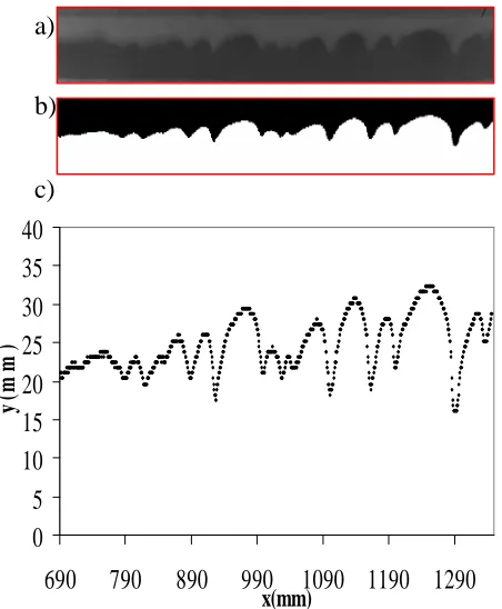
In this section, we present a study of the spatiotemporal dynamics of CAF interface. The spatiotemporal diagram technique is used to extract the evolution of interface of CAF. The images have a variation of light intensity I(x, y) (see fig. 7-a), where the up region represents the oil phase while the down region represents the water. To perform an automatic extraction of the evolution of interface of CAF, we developed the spatiotemporal diagram technique from the images recorded by the camera. To distinguish the position of the interface of CAF in time, we used the binarization technique of each image: The resulting signal I was normalized by its maximal intensity: i =I/Im. The cutoff ∆ that reproduces the discharge evolution was found at 0.5. We assigned black color (i < ∆) to oil phase and white (i > ∆) to water phase (Fig. 7-b).

Fig.7. Image interface of water-oil: (a) raw image, (b) digitized image; (c) spatial profile.

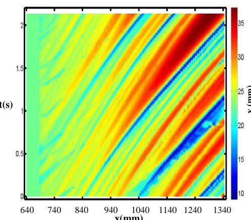
We developed a program in Matlab in order to extract automatically the position of the interface of CAF in the time from binarized spatiotemporal diagram. We extracted the spatial profile of the interface y(x) from binarized intensity I(x,y) for each image along the longitudinal and depth directions (Fig. 7-c). The chronological superposition of these spatial profiles at regular intervals (0.032s) permits to provide a spatiotemporal diagram of the position of the interface y (x, t): The vertical axis is the time t, the horizontal axis the distance x from the inlet and the position y (x, t) of the interface is encoded into a color level. A typical spatiotemporal diagram of interface oil-water is displayed in figure 8. The homogeneous color level close to the inlet corresponds to a region of constant y (parallel flow

a)

b)

c)

0

5

10

15

20

25

30

35

40

690

790

890

990

1090 1190 1290

x(mm)

y

(m

m

)

0.2 0.25 0.3 0.35 0.4 0.45 0.5

Qw(l/s) L|| /h 30 32 34 36 38 40 42

0.25 0.3 0.35 0.4 0.45 0.5

Qw(l/s)

L

||

the previous section). Further downstream, one can observe stripes with blue color for low undulation of CAF and red color for high undulation of CAF, the slope and color of which give the velocity and the amplitude of the instability waves.

The interface location can be described by the following equation:

y (x,t)= A(x,t) exp(i(qx -2πft)) +c.c (1) where A(x,t) is the spatiotemporal amplitude, q(x,t) is the spatiotemporal wave number, and f(x,t) is the spatiotemoral frequency.

Fig. 8. Spatiotemporal diagram of interface oil-water.

In figure 9, we plot the time dependence of y (t) for four different positions x along the channel length. As expected for a spatially unstable regime, we observe, downstream the inlet, an increase of the amplitude of the fluctuations. Figure 10 shows the spatial amplitude A(x) of unstable CAF averaged in time. The amplitude profile of figure 10 shows a three zones: i) zone with vanishing amplitude, which correspond to the parallel CAF without instability, ii) zone of spatial growth rate, where the amplitude increases with space, it corresponds to growing instability, iii) zone of amplitude saturation where the amplitude is almost constant with small fluctuations. In order to extract the evolution of frequency from the spatiotemporal diagram, we superpose the power spectra of frequency at different space positions x: the vertical axis represents frequency, the horizontal axis represents the position x and the power spectrum is encoded in color scale. Such a typical diagram is given in figure 11. As in the spatiotemporal diagram, we can observe the strong dependence of frequency to the space x. We observe also the presence of harmonic modes in power spectrum which is the signature of a strong non-linear interface of CAF. Figure 12 shows frequency power spectrum measured at x= 1321 mm i.e. at the zone of amplitude saturation. The frequency power spectrum (fps) is

maximum

Fig. 9. Temporal variation of interface y(x,t) at four different position x.

Fig.10. Spatial amplitude diagram of interface oil-water.

In order to extract the evolution of frequency from the spatiotemporal diagram, we superpose the power spectra of frequency at different space positions x: the vertical axis represents frequency, the horizontal axis represents the position x and the power spectrum is encoded in color scale. Such a typical diagram is given in figure 11. As in the spatiotemporal diagram, we can observe the strong dependence of frequency to the space x. We observe also the presence of harmonic modes in power spectrum which is the signature of a strong non-linear interface of CAF. Figure 12 shows frequency power spectrum measured at x= 1321 mm i.e. at the zone of amplitude saturation. The frequency power spectrum (fps) is characterized by the frequency fmax at which the fps is

maximum.

t(s)

640 740 840 940 1040 1140 1240 1340

x(mm) y ( m m )

0 10 20 30 40 50 60 70 80 90

0 2 4 6 8 1 0 1 2 1 4 1 6 1 8 2 0 2 2 2 4 2 6 26 24 22 20 18 16 14 12 10 8 6 4 2 0 t(s)

700 907 1114 1321 x (mm)

0 2 4 6 8 10 12 14 16

0 200 400 600 800 1000 1200 1400

x(mm) A ( m m )

Parallel CAF

Fig.11. Spatial frequency variation, where the power spectrum is coded in color.

Fig.12. Power spectrum of frequency at the zone of the saturation of amplitude.

The characteristics of the interface wave of CAF (fmax:

frequency maximum, λ: wavelength As: amplitude is saturation zone and the wave speed or phase velocity) are summarized in figure 13.

From, the figure 13, we remark that the frequency, wave speed and the saturation amplitude increase with Qw, while the wavelength decreased as function as Qw from Qw=0.25 l/s to 0.45 l/s. The evolution of pressure drop with flow rate of water is presented in figure 14. The pressure drop decreases with the flow rate of water. In comparison with different characteristics of CAF in parallel or in saturation zones, we can conclude that the pressure drop follows the

same

Conclusion

In this work, we studied the stability of the interface of CAF in an oil-water system at fixed oil flow rate (Qo=0.19 l/s) and varied flow rate of water Qw. We found that for large values of Qw (typically Qw>0.23l/s), CAF is unstable, and it becomes stable for the low values of Qw (typically Qw<0.23l/s). We showed that CAF strongly depends on space x and we could measure parallel length L||, amplitude and frequency in space. The pressure drop decreased with water flow rate. This behavior is similar to that of the oil core height (hoil), L|| and λwavelength of CAF interface and it is opposite to that of saturation amplitude As, maximum frequency fmax and wave speed c.

P

ow

er

S

p

ec

tr

u

Fig.13. Variation of the characteristics the interface wave of CAF with Qw at fixed Qo=0.19 l/s a) fmax: frequency maximum, b) λ:

wavelength; c) c: wave speed or phase velocity and As: saturation amplitude.

3.00 3.20 3.40 3.60 3.80 4.00 4.20 4.40 4.60 4.80

0.2 0.25 0.3 0.35 0.4 0.45 0.5

Qw(l/s)

∆∆∆∆

p

/L

(b

a

r/

m

)

Fig.14. Variation of pressure drop of CAF with Qw at fixed

Qo=0.19 l/s

a)

_b)

120 140 160 180 200 220

0.25 0.3 0.35 0.4 0.45 0.5

Qw(l/s)

λ λ λ λ

(m

m

)

0.6

0.8

1

1.2

1.4

0.25

0.3

0.35

0.4

0.45

0.5

Q

(

l

/s)

f

a

x

(h

z

)

d)

100 140 180 220 260

0.25 0.3 0.35 0.4 0.45 0.5

Qw(l/s)

c

(m

m

/s

)

-2 0 2 4 6 8 10 12 14 16

0.25 0.3 0.35 0.4 0.45 0.5

Qw(l/s)

As

(

m

m

)

References

1. T. Russell, G. Hodgson and G. Govier, Can. J. Chem. En. 37, 9 (1959)

2. A. Huang and D. Joseph, J. Fluid. Mech. 282, 233-245 (1995)

3. R. Oliemans, G. Ooms, Core-annular flow of oil and

water through a pipe line, Multiphase science and

Technology (Hemisphere, Vol 2, New York, 1986). 4. A. Bensakhria, Y. Peysson, G. Antonini, OilGas Sci

Technol Rev IFP 59 5, 523-33 (2004)

5.

6.

7. P. Guillot, A. Colin, AS. Utada, A. Ajdari, Phys Rev Lett. 99, 104502 (2007).

8. D. Joseph, M. Renardy, Y. Renardy, J Fluid Mech

141, 309-17 (1984)

9. D. Joseph, M. Renardy, Fundamentals of two-fluid

dynamics (Springer, New York, 1993)

10. T. Kao, C. Park, J Fluid Mech 52, 401-23 (1972)

11.