Quaternion-Based Iterative Solution of Three- Dimensional Coordinate Transformation Problem

(1)

Quaternion-Based Iterative Solution of

Three-Dimensional Coordinate Transformation

Problem

Huaien Zeng and Qinglin Yi

College of Civil Engineering and Architecture, China Three Gorges University, Yichang, China [email protected]

Abstract—Three-dimensional coordinate transformation

problem is the most frequent problem in photogrammetry, geodesy, mapping, geographical information science (GIS), and computer vision. To overcome the drawback that traditional solution of the problem based on rotation angles depends strongly on initial value of parameter, which makes the method ineffective in the case of super-large rotation angle, the paper adopts an unit quaternion to represent three-dimensional rotation matrix, then puts forward a quaternion-based iterative solution of the problem. The cases study shows that the quaternion-based solution has no dependence on the initial value of parameter and desirable result with fast speed. Thus it is valid for three-dimensional coordinate transformation of any rotation angle.

Index Terms—three-dimensional coordinate transformation,

quaternion, rotation matrix, initial value of parameter, parameter adjustment with constraint, improved Gauss-Newton method

I. INTRODUCTION

Three-dimensional (3D) coordinate transformation is the most common issue in geodesy, photogrammetry, geographical information science (GIS), computer vision and other research areas. It involves transforming spatial data (locations, images, maps, etc.) from an original coordinate system to a target coordinate system by means of mathematical transformation model. Presently, the most frequently model is the similarity transformation model with seven parameters (namely, one scale factor, three translation parameter, and three rotation angles.), also known as Helmert or conformal group C7(3)

transformation, which is employed in the paper. To carry out coordinate transformation, it is critical to calculating the seven parameters, usually by some control points with the coordinates in the both systems.

In geodesy, because the rotation angles are generally very small, namely the two coordinate systems are nearly aligned; the similarity transformation model is simplified to a linear one (e.g., [1]-[2]), whose parameters are easy to solve. A lot of literatures on coordinate transformation from World Geodetic System 1984 (WGS84) to a local system have been published (e.g., [2]-[5]). It is notable

that [5] presented a stepwise approach to individually calculate the seven parameters by the geometric properties of similarity transformation.

In photogrametry and computer vision, three-dimensional coordinate transformation is employed to relate image space coordinates to object space coordinates in the so-called “absolute orientation” problem ([6]) or to register multi-station point clouds in a LIDAR surveying ([7]). In these cases, the rotation angles are almost not small and require the solution of nonlinear three-dimensional coordinate transformation model.

Many algorithms have been presented to compute the transformation parameters from the nonlinear over-determined equations of coordinate transformation in least-squares (LS) sense. They can be divided into two categories, i.e., iterative algorithms and analytical algorithms. The former are dominant, e.g., [8]-[11]. The major difference between these algorithms is caused due to the different representations of rotation matrix, which lead to the different linearization models. However, the iterative algorithms traditionally need good initial starting values of parameters and linearization process. It is difficult to implemented in the cases of large rotation angles because the initial values are difficult even impossible to get in advance. At present, the analytical algorithm is rarely seen, of which two key algorithms are presented, known as the Procrustes algorithm ([12]) and a quaternion-based algorithm ([13]). The authors presented a new analytical algorithm based on optimization process and the good properties of Rodrigues matrix ([14]).

To solve the problem that traditional algorithms with the mathematical model based on rotation angles depend strongly on the initial values of parameters, and calculate slowly because of the existing numerous trigonometric computation, the paper will investigate the feasibility of coordinate transformation model with representation of quaternion, and present a efficient algorithm to compute the transformation parameters.

The remainder of the paper is organized as follows. Section II briefly reviews the concept and properties of quaternion, and then derives the representation of rotation matrix by unit quaternion. Section III derives the mathematical model of 3D coordinate transformation inverse problem based on unit quaternion in detail, and presents the solution of transformation parameters. In order to speed up the convergence of iterative calculation,

This work is supported by Youth Science Foundation of China Three Gorges University (No.KJ2009A004) and Talent Research Start-up Fund of China Three Gorges University (No.KJ2009B008).

(2)

we design an improved Gauss-Newton method to substitute the most frequently used classical Gauss-Newton method in the adjustment of geodetic photographic data, etc. The simulative and practical cases are studied to validate the presented algorithm in the next two sections, i.e., Sect. IV and Sect. V respectively. Finally, conclusions are made in Sect. VI.

II. QUATERNION AND 3DROTATION MATRIX

A. Concept and Properties of Quaternion

Quaternion was a mathematic concept invented by Hamilton in 1843, which is represented as follows [15].

Q

= +

q

₁

iq

₂

+

jq

₃

+

kq

₄

,

(1)

where

q

₁ is the real part,

q

₂ ,

q

₃ and

q

₄ are the imaginary part,

i

,

j

and

k

are imaginary units, and they meet the relationships: ①

i

2

=

j

2

=

k

2

= −

1

, ②

ij

= − =

ji

k

, ③

jk

= − =

kj

i

, ④

ki

= − =

ik

j

. The corresponding conjugate quaternion can be denoted as

*

1 2 3 4

.

Q

= −

q

iq

−

jq

−

kq

(2) In order to simplify the description,

Q

is expressed as

(

1

)

T T

q

in the column vector form with respect to the

bases

(

1 i

j

k

)

, where

(

2 3 4

)

T

q

=

q

denotes a 3D vector ,

q

₁ denotes a scalar, and

T

the transpose. The norm of quaternion

Q

is defined as

Q

=

q

₁2

+

q

₂2

+

q

₃2

+

q

₄2

.

(3)

If

Q

=1,

Q

is called unit quaternion.

According to the definition of quaternion, it is easily proved that the following properties are satisfied for quaternion

(

₁ ₁ T T

)

T

,

P Q

+ =

p

+

q

p

+

q

(4)

1 1 1 1

,

PQ

=

p q

− ⋅ + × +

p q

+

q p

(5)

(

)

(

)

OPQ

=

OP Q

=

O PQ

, (6)

(

)

O P Q

+

=

OP OQ

+

, (7)

(

OP

)

∗

=

P O

∗ ∗ , (8)

QQ

∗

=

Q

, (9)

1

Q

−

=

Q

∗

Q

, (10) where

O

,

P

and

Q

are quaternions,

Q

−1 denotes the inverse of the quaternion

Q

, and the symbols

⋅

and

×

stand for the dot product and cross product, respectively. The dot and cross product of vectors are defined as

T

p q

⋅ =

p q

, (11)

( )

p q

× =

c p q

, (12) where

4 3

4 2

3 2

0 ( )

0

0 p

p

c p

p

−

⎡

⎤

⎢

⎥

=

_⎢

−

_⎥

⎢

−

⎥

⎣

⎦

. (13)

The product quaternion

PQ

can be expressed in the column vector and matrix form as

PQ

=

C P Q

( )

=

C Q P

( ) ,

(14)

where

1 1

( )

T

p

C P

p

p I

c p

⎡

−

⎤

= ⎢

₊

⎥

⎣

⎦

,

1 1

( )

T

q

C Q

q

q I

c q

⎡

−

⎤

= ⎢

₋

⎥

⎣

⎦

, and

I

denotes a 3×3

identity matrix.

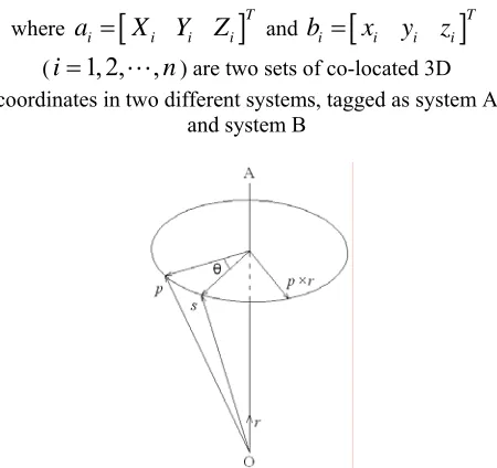
B. 3D Rotation Matrix Represented by Quaternion Supposing vector

s

is produced of vector

p

by means of rotation angle of

θ

around axis OA, and the OA-axis unit vector is

r

(see Fig. 1), a well-known method to represent the rotation of

p

to

s

is derived with quaternion [16]

S

=

QPQ

*

=

C Q C Q P

( ) (

*

) ,

(15)

where

P

and

S

are the quaternion forms of vectors

p

and

s

with scalar both as zero,

Q

is a unit quaternion formed by

θ

and

r

as

Q

=

cos( / 2)

θ

+

r

sin( / 2),

θ

(16).

where,

r

= +

ir

₁

jr

₂

+

kr

₃, and

r

₁2

+

r

₂2

+

r

₃2

=

1

.

*

( ) (

)

C Q C Q

in (16) can be expanded as

1 0

0 R

⎡

⎤

⎢

⎥

⎣

⎦

,

where

(

₁2 T

)

2 (

T ₁

( ) .

)

R

=

q

−

q q I

+

qq

+

q c q

(17)

R

in (17) is the 3D rotation matrix, whose elements are composed of the unit quaternion

Q

.

III. QUATERNION-BASED ITERATIVE SOLUTION OF 3D

COORDINATE TRANSFORMATION PROBLEM

A. Mathematic Model

The seven-parameter similarity transformation model can be expressed as [2]

(3)

where

a

_i

=

[

X

_i

Y

_i

Z

_i

]

T and

b

_i

=

[

x

_i

y

_i

z

_i

]

T (

i

=

1, 2, ,

"

n

) are two sets of co-located 3D coordinates in two different systems, tagged as system A

and system B

Figure 1. Rotation of vector and the physical meaning of quaternion

respectively,

t

= ∆

[

X

∆

Y

∆

Z

]

T denotes three translation parameters,

λ

denotes the scale parameter and

R

denotes the 3×3 rotation matrix, which contains the three rotation angles. It is Obvious that in order to determine the seven parameters, the number

n

of co-located coordinates

a

_i,

b

_i must be greater than or equal to three.

If we substitute (17) into (18), we can obtain the quaternion-based non-linear 3D coordinate transformation model. In terms of linearization of the model, we obtain the observation equation. However, the corresponding normal equation in actual adjustment usually doesn’t avoid ill-posed property. For this reason, we transform (18) to another form by means of baseline vector, namely difference of coordinates which eliminates the three translation parameters as follows

∆ =

a

i

λ

R b

∆

i

,

(19)

where

∆ = −

a

i

a

i

a

₀

,

∆ = −

b

i

b

i

b

0,

a

0 and

b

0 denote

two sets of co-located 3D coordinates for the starting point of all baselines, and the starting point can be often supposed to be a point with high accuracy. By means of linearization of (19), the observation equation are obtained as follows

V

i

=

B x l

i

δ

−

i

,

(20)

where

V

_i

= ⎣

⎡

V

_xi

V

_yi

V

_zi

⎤

_⎦

T denotes correction of

i

a

∆

,

δ

x

=

[

dq

₁

dq

₂

dq

₃

dq

₄

d

λ

]

T denotes

correction of unkowns

x

=

[

q

₁

q

₂

q

₃

q

₄

λ

]

T ,

i

B

is a 3×5 coefficient matrix as

11 12 13 14 1

21 22 23 24 2

31 32 33 34 3

i

B

K

B

K

B

K

⎡

⎤

⎢

⎥

= ⎢

⎥

⎢

⎥

⎣

⎦

, (21)

T

i xi yi zi

l

= ⎣

⎡

l

⎤

_⎦

is a constant matrix, and the elements of

B

_i and

l

_i are listed in Appendix A.

Because

Q

is a unit quaternion, there is a constraint accompanying (20) as follows

q

₁2

+

q

₂2

+

q

₃2

+

q

₄2

=

1.

(22)

Linearizing (22), we obtain

C x W

δ

−

x

=

0,

(23) where

[

1 2 3 4

0 ,

]

C

=

q

2 2 2 2

1 2 3 4

(1

) 2.

x

W

= −

q

−

q

−

q

−

q

B. Classical Solution of the Transformation Parameters When the number of co-located points

n

≥

3

, we can establish

3(

n

−

1)

observation equations like (20) as

,

V

=

B x l

δ

−

(24)

where

1

1 n

V

₋

⎡

⎤

⎢

⎥

= ⎢ ⎥

⎢

⎥

⎣

⎦

#

,

1

1 n

B

₋

⎡

⎤

⎢

⎥

= ⎢ ⎥

⎢

⎥

⎣

⎦

#

,

1

1 n

l

₋

⎡

⎤

⎢

⎥

= ⎢ ⎥

⎢

⎥

⎣

⎦

#

, with a

constraint, i.e., (23). Then we can solve the transformation parameters by means of parameter adjustment with constraint [17], and the expression of solution

δ

x

can be written as

1 1 1 1 1 1

(

)

bb bb cc bb bb cc

T T

x

N

N C N CN

W

N C N W

δ

₌

−

₋

− − −

₊

− −

(25)

where T

,

bb

N

=

B

Σ

B

T

W

=

B

Σ

l

, T

,

cc bb

N

=

CN C

Σ

denotes the weight matrix of observations. To simplify the calculation, in this paper we suppose the weight matrix of observations is an identity matrix, namely

Σ =

I

.

Because it is difficult or even impossible to get the initial value (i.e., approximation) of parameter in advance, the classic Gauss-Newton method (see [18]) is usually employed to solve the parameters iteratively, i.e., we firstly give rough approximation of

x

, then solve the correction

δ

x

by means of parameter adjustment with constraint (using (25)), and give the approximation of

x

of next iteration as

x

+

δ

x

, then repeat the above procedure until the

δ

x

is less than a given tolerance, or other termination conditions are satisfied.

(4)

because of iterative non-convergence. For the sake, a improved Gauss-Newton method is presented, which uses the k-th iterative solution k

x

δ

of classic Gauss-Newton method, then adds a adaptive variable step-size k

s

in the next iteration as follows

k 1 k k k

,

x

+

=

x

+

s

δ

x

(26) which satisfies T

(

k 1

) (

k 1

)

T

( ) ( )

k k

V

x

+

V x

+

<

V

x V x

, where

( )

k

V x

is the k-th iterative correction of coordinates. The calculation formula of k

s

is as follows [19]

0.5 0.25[ ( )

(

)]/

[ ( )

(

) 2 (

0.5 )],

k k k k

k k k k k

s

R x

x

R x

x

R x

x

δ

=

+

−

+

−

+

(27) where

( )

k

R x

is k-th iterative objective function as follows

( )

k T

( ) ( ) 2

k k T

( ) ( ),

k k

R x

=

f

x

f x

−

f

x l x

(28) where

1

( )

k

k n

f x

f

₋

x

⎡

⎤

⎢

⎥

= ⎢

⎥

⎢

⎥

⎣

⎦

#

,

( )

k k k

,

i i i

f x

= ∆ −

a

λ

R

∆

b

1

( )

k

k n

l x

l

₋

x

⎡

⎤

⎢

⎥

= ⎢

⎥

⎢

⎥

⎣

⎦

#

,

( )

k i

l x

is the k-th iterative

l

_i ,

(

i

=

1, 2, ,

"

n

−

1

).

The quaternion-based solution of non-linear 3D coordinate transformation parameters (hereinafter, “quaternion method”) is finally summarized as

Step 1. Initiate

x

, e.g., set the initial value of

λ

to 1, and the initial values of

q

₁,

q

₂,

q

₃ and

q

₄ to 0.5 respectively, or set one of them to 1 and the others to 0.

Step 2. Establish observation equation and constraint equation, and solve

δ

x

by means of parameter adjustment with constraint (using (25)), if every element of

δ

x

is less than given tolerance

τ

(in this paper,

τ

is given 1.0×10-9_{), turn to Step 5.}

Step 3. Firstly Compute

( )

k

R x

by using (28), then compute k

s

by using (27), lastly compute k 1

x

+ by using (26).

Step 4. Calculate

(

k 1

)

R x

+ by using (28), and if

1

(

k

)

( )

k

,

R x

+

−

R x

<

ε

where

ε

is a given tolerance, (in the paper, it is set to 1.0×10-9_{), turn to Step 5, else}

initiate

x

with k 1

x

+ , continue Step 2.

Step 5. Substitute the solution of

x

and the coordinates

a

₀ and

b

₀ into (18), obtain

t

, finally output

x

and

t

.

Substituting the solution of the unit quaternion

Q

into (17), we obtain the rotation matrix

R

. Supposing

R

is formed by rotating angles

α

,

β

,

γ

counterclockwise around the Cartesian X, Y and Z axes respectively, then

R

can be expressed by rotation angles as

cos cos

sin cos

cos sin sin

sin sin

cos sin cos

sin cos

cos cos

sin sin sin

cos sin

sin sin cos

.

sin

cos sin

cos cos

R

γ

β

γ

α

γ

β

α

γ

α

γ

β

α

γ

β

γ

α

γ

β

α

γ

α

γ

β

α

β

α

β

α

+

−

⎡

⎤

⎢

⎥

= −

_⎢

−

+

_⎥

⎢

−

⎥

⎣

⎦

(29)

Using (29), the rotation angles

α

,

β

,

γ

can be computed as

1 32 1 1 21

31

33 11

tan

R

,

sin (

R

),

tan

R

α

_{= −}

−

β

₌

−

γ

_{= −}

− _.

(30) where

R

_ij is the element of

R

in the i-th row and j-th column.

If we substitute (29) into (19), we obtain the transformation model based on rotation angle. Further we can also establish the observation equation with the rotation angle in terms of linearization, and gain the least squares solution by means of parameter adjustment. Similarly to the 5 steps of quaternion method, finally we can get solution of the seven transformation parameters. This method is the classical one based on rotation angle (hereinafter, “angle algorithm”).

IV. SIMULATIVE CASE STUDY AND DISCUSSION

The simulative data and demonstrative process are made as follows. Firstly, the simulative true values of coordinates in system B and transformation parameters are given. Secondly, coordinates in system A (simulative true values) are computed by using (18). Thirdly, the transformation parameters (calculated values) are solved with quaternion method using the above simulative coordinates. Finally, the correctness of the method is proved by comparing the calculated values and simulated values of the parameters and the transformation residuals of coordinates.

Simulated true values of coordinates in system B in system A are listed in Table I. The simulative transformation parameters have three sets, tagged as set 1, set 2, and set 3 corresponding small rotation angle, large rotation angle and super-large rotation angle in Table II. Simulated true values of coordinates in system A are listed Table III.

(5)

point 1, 2, 4, 6, 8, (the other four points are reserved for residual calibration of coordinate), we obtain the result as shown in Table IV. To compare quaternion method with angle method, the solution of angle method is also listed in Table IV. The transformation residuals of coordinates in Table IV (using all 9 points) are the differences between the simulative true values and calculated values of coordinates in system A, of which the latter is obtained by substituting coordinates in system B and calculated transformation parameters into (18).

It is clearly seen in Table IV that although the errors and transformation residuals get larger and larger with the increase of rotation angles (from set 1 to set 2 and to set 3), it doesn’t change the validation of the quaternion method (all the errors and residuals are too small to be neglectable), and the iteration keep a fast speed (9 to 11 times) regardless of the increase of rotation angles. For small and large angles transformation (set 1 and set 2), rotation angle method is correct, and its solution speed is fast (less than 16 times), but for super large angle transformation (set 3), it can not solve the parameters because of its strong dependence on initial values of parameters.

To validate the superiority of the improved Gauss-Newton method to the classic Gauss-Gauss-Newton method, the iterative process of them are compared in Fig. 2. The left column is about the relationship of step-size with iteration times, and the right column is about the relationship of objective function with iteration times in Fig. 2. As seen in Fig. 2, for small angle case (set 1), the classic Gauss-Newton method failed after iterative 30 times, showing divergent trend, and with two fluctuations in a few steps of iteration, but the improved Gauss-Newton method converged after iterative 11 times, and with no fluctuations. For large angle case (set 2), the classic Gauss-Newton method succeeded in convergence after iterative 13 times with fluctuations in a few steps of iteration, however the improved Gauss-Newton method converged after iterative 11 times, and with no fluctuations. For super large angle case (set 3), the classic Gauss-Newton method succeeded in convergence after

iterative 18 times with fluctuations, however the improved Gauss-Newton method converged after iterative 9 times with no fluctuations. The analysis above indicates that the adaptive step-size strategy is very important, which accelerates the convergence rate and avoids the iterative fluctuation. Thus, the improved Gauss-Newton method is valid compared to the classic Gauss-Newton method.

V. ACTUAL CASE STUDY AND DISCUSSION

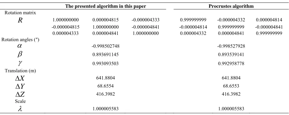
In order to demonstrate the application of the presented algorithm in the paper and compare it with the famous Procrustes algorithm presented by E. W. Grafarend and J. L. Awange (see [12]), an actual case is investigated in this section. The Cartesian coordinates of seven stations, as listed in Table V, are taken from [12]. Using these coordinates, the transformation parameters are computed with the presented algorithm, as shown in Table VI. In the process, the barycenter of all seven stations is selected as the starting point of baselines to keep consistence with [12]. To compare with the Procrustes algorithm, the results reported in [12] are also listed in Table VI. The rotation angles corresponding to the Procrustes algorithm are not directly obtained from [12] but calculated by the authors according to the computed result of rotation matrix. The residuals are given in Table VII.

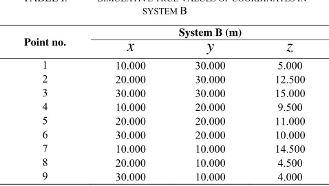
TABLE I. SIMULATIVE TRUE VALUES OF COORDINATES IN SYSTEM B

Point no.

_x

System B (m)

_y

_z

1 10.000 30.000 5.000

2 20.000 30.000 12.500

3 30.000 30.000 15.000

4 10.000 20.000 9.500

5 20.000 20.000 11.000

6 30.000 20.000 10.000

7 10.000 10.000 14.500

8 20.000 10.000 4.500

9 30.000 10.000 4.000

TABLE II. SIMULATIVE TRUE VALUES OF TRANSFORMATION PARAMETERS

Set no.

∆

X

(m)

∆

Y

(m)

∆

Z

(m)

α

β

γ

λ

Set 1 30 30 10 47′ 32′ 55′ 1.000016

Set 2 30 30 10 27° 21° 24° 1.000016

Set 3 30 30 10 71° 78° 73° 1.000016

TABLE III. SIMULATIVE TRUE VALUES OF COORDINATES IN SYSTEM A

Point no.

_x

System A (Set 1) (m)

_y

_z

System A (Set 2) (m) System A (Set 3) (m)

X

Y

Z

X

Y

Z

(6)

TABLE IV. DIFFERENCES BETWEEN CALCULATED VALUES AND SIMULATIVE TRUE VALUES OF TRANSFORMATION PARAMETERS

Transformation Parameters

Set 1 Set 2 Set 3

Quaternion method

Angle method

X

∆

(m) 3.8×10-10 5.2×10-6 4.6×10-7 -5.7×10-6 4.4×10-7

Y

∆

(m) -7.9×10-11 -9.2×10-7 8.3×10-8 -2.2×10-5 1.8×10-7

Z

∆

(m) -2.7×10-10 -3.3×10-6 7.1×10-8 -6.3×10-6 1.2×10-7

α

(″) -1.5×10-6_-3.2×10-2_-7.7×10-4_-5.8×10-2_-1.4×10-3

β

₍_″₎ 9.4×10-7_-2.7×10-2_5.0×10-5_2.6×10-2_-9.1×10-4

γ

₍_″₎ -2.4×10-6_-3.8×10-2_-1.9×10-3_-6.3×10-2_4.0×10-3

λ

-3.0×10-13_-1.0×10-8_-1.1×10-8_5.7×10-7_-5.6×10-9

max. order of magnitude

of residuals (m) 10

-10₁₀-6₁₀-7₁₀-5₁₀-7

Iteration times 11 12 11 16 9 divergence

0 5 10 15 20 25 30

0.2 0.4 0.6 0.8 1 1.2

Iteration times

S

teps

iz

e

Set 1

classic Gauss-Newton method improved Gauss-Newton method

0 5 10 15 20 25 30

-20 -15 -10 -5 0 5

Iteration times

lo

g10

(V

TV)

Set 1

0 2 4 6 8 10 12 14

0.2 0.4 0.6 0.8 1 1.2 1.4 1.6

Iteration times

S

teps

iz

e

Set 2

0 2 4 6 8 10 12 14

-15 -10 -5 0 5

Iteration times

lo

g10

(V

TV)

Set 2

0 2 4 6 8 10 12 14 16 18

0.5 0.6 0.7 0.8 0.9 1 1.1 1.2

Iteration times

S

teps

iz

e

Set 3

0 2 4 6 8 10 12 14 16 18

-15 -10 -5 0 5

Iteration times

lo

g10

(V

TV)

Set 3

Figure 2. Iterative process comparison of the improved Gauss-Newton method with the classic Gauss-Newton method

TABLE V. CARTESIAN COORDINATES IN SYSTEM B AND A

Station Name

_x

System B (local system) (m)

_y

System A (WGS-84) (m)

z

X

Y

Z

(7)

Ex Mergelaec 4137012.190 671808.029 4791128.215 4137659.549 671837.337 4791592.531 Ex Hof Asperg 4146292.729 666952.887 4783859.856 4146940.228 666982.151 4784324.099 Ex Kaisersbach 4138759.902 702670.738 4785552.196 4139407.506 702700.227 4786016.645

TABLE VI. TRANSFORMATION PARAMETERS RESULTS OF THE PRESENTED ALGORITHM IN THIS PAPER AND I-LESS PROCRUSTES ALGORITHM

The presented algorithm in this paper Procrustes algorithm

Rotation matrix

R

1.000000000 0.000004815 -0.000004333 0.999999999 -0.000004332 0.000004814 -0.000004815 1.000000000 -0.000004841 -0.000004814 0.999999999 -0.000004841

0.000004333 0.000004841 1.000000000 0.000004332 0.000004841 0.999999999

Rotation angles (″)

α

-0.998502748 -0.998527928

β

0.893691145 0.893539141

γ

0.993093503 0.992958778

Translation (m)

X

∆

641.8804 641.8804

Y

∆

68.6554 68.6553

Z

∆

416.3982 416.3982

Scale

λ

1.000005583 1.000005583

TABLE VII. TRANSFORMATION RESIDUALS OF THE PRESENTED ALGORITHM IN THIS PAPER AND I-LESS PROCRUSTES ALGORITHM (M)

The presented algorithm in this paper Procrustes algorithm

Station Name

_X

_Y

_Z

_X

_Y

_Z

Solitude 0.0940 0.1351 0.1402 0.0940 0.1351 0.1402

Buoch Zeil 0.0588 -0.0497 0.0137 0.0588 -0.0497 0.0137

Hohenneuffen -0.0399 -0.0879 -0.0081 -0.0399 -0.0879 -0.0081

Kuehlenberg 0.0202 -0.0220 -0.0874 0.0202 -0.0220 -0.0874

Ex Mergelaec -0.0919 0.0139 -0.0055 -0.0919 0.0139 -0.0055

Ex Hof Asperg -0.0118 0.0065 -0.0546 -0.0118 0.0065 -0.0546

Ex Kaisersbach -0.0294 0.0041 0.0017 -0.0294 0.0041 0.0017

VI. CONCLUDING REMARKS

To overcome the drawback that angle method depends strongly on initial value of parameter, especially on rotation angles, which makes the method ineffective in the case of super-large rotation angle due to the beyond estimation in advance, this paper uses quaternion to represent 3D rotation matrix, then presents the quaternion-based iterative method in terms of linearization. The iterative method designs an adaptive step-size based on the classic Gauss-Newton method, which accelerates the convergence rate and avoids the iterative fluctuation. The cases study shows that the method has no dependence on initial value of parameter and satisfactory result with fast speed, and is suitable for coordinate transformation of any rotation angle.

APPENDIX THE ELEMENTS OF

B

_i AND

l

_i

11

2 (

4 i 3 i

)

B

=

λ

− ∆ + ∆

q

x

q

z

,

12

2 (

3 i 4 i

)

B

=

λ

q

∆ + ∆

y

q

z

,

13

2 ( 2

3 i 2 i 1 i

)

B

=

λ

−

q

∆ + ∆ + ∆

x

q

y

q z

,

14

2 ( 2

4 i 1 i 2 i

)

B

=

λ

−

q

∆ − ∆ + ∆

x

q y

q

z

,

21

2 (

4 i 2 i

)

B

=

λ

q

∆ − ∆

x

q

z

,

22

2 (

3 i

2

2 i 1 i

)

B

=

λ

q

∆ −

x

q

∆ − ∆

y

q z

,

23

2 (

2 i 4 i

)

B

=

λ

q

∆ + ∆

x

q

z

,

24

2 (

1 i

2

4 i 3 i

)

B

=

λ

q x

∆ −

q

∆ + ∆

y

q

z

,

31

2 (

3 i 2 i

)

B

=

λ

− ∆ + ∆

q

x

q

y

,

32

2 (

4 i 1 i

2

2 i

)

B

=

λ

q

∆ + ∆ −

x

q y

q

∆

z

,

33

2 (

1 i 4 i

2

3 i

)

B

=

λ

− ∆ + ∆ −

q x

q

y

q

∆

z

,

34

2 (

2 i 3 i

)

B

=

λ

q

∆ + ∆

x

q

y

,

2 2

1 3 4 2 3 1 4

1 3 2 4

[1 2(

)]

2(

)

2(

)

i i

i

K

q

x

q q

y

q q

z

= −

+

∆ +

−

∆

+

∆

,

2 2

2 1 4 2 3 2 4

3 4 1 2

2(

)

[1 2(

)]

2(

)

i i

i

K

q q

x

q

y

q q

z

=

+

∆ + −

+

∆

+

−

∆

,

3 2 4 1 3 1 2 3 4

2 2

2 3

2(

)

2(

)

[1 2(

)]

i i

i

K

q q

x

q q

y

q

z

=

−

∆ +

+

∆

+ −

+

∆

,

1

xi i

l

= ∆ −

X

λ

K

,

2

yi i

l

= ∆ −

Y

λ

K

,

3

zi i

(8)

ACKNOWLEDGMENT

The authors thank Prof. S. X. Huang of School of Geodesy and Geomatics, Wuhan University for his valuable comments and suggestions, which enhanced the quality of this manuscript. The first author is grateful to the support and good working atmosphere provided by his research team in China Three Gorges University.

REFERENCES

[1] A. Leick, GPS satellite surveying, 3rd edn. Wiley, Hoboken, 2004.

[2] Y. Z. Shen, L. M. Hu, and B. F. Li, “Ill-posed problem in determination of coordinate transformation parameters with small area’s data based on Bursa model,” Acta Geod. et Cartogr. Sinica, vol.35, no.2, pp.95-98, May 2006 (in

Chinese).

[3] T. Soler, and R. A. Snay, “Transforming positions and velocities between the International Terrestrial Reference Frame of 2000 and North American Datum of 1983.” J. Surv. Eng., 130(2), 49-55, 2004.

[4] I. Kashani, “Application of generalized approach to datum transformation between local classical and satellite-based geodetic networks”. Surv. Rev., vol.38, no.299, pp.412–

422, 2006.

[5] J. Y. Han, H. W. B. Van Gelder, “Step-wise parameter estimations in a time-variant similarity transformation”. J. Surv. Eng. 132(4):141–148, 2006.

[6] E. M. Mikhail, J. S. Bethel, C. J. McGlone, Introduction to modern photogrammetry. Wiley, Chichester, 2001.

[7] J. J. Jaw , and T. Y. Chuang, “Registration of ground-based LIDAR point clouds by means of 3D line features” J. Chinese Inst. of Eng., 31(6), 1031-1045, 2008.

[8] W. X. Zeng and B. Z. Tao, “Non-linear adjustment model of three-dimensional coordinate transformation”,

Geomatics and Information Science of Wuhan University,

vol.28, no.5, pp.566-568, Oct. 2003 (in Chinese).

[9] Y. Chen, Y. Z. Shen, D. J. Liu, “A simplified model of three dimensional-datum transformation adapted to big rotation angle”, Geomatics and Information Science of Wuhan University, vol.29, no.12, pp.1101-1105, Dec.

2004 (in Chinese).

[10]J. L. Yao, B. M. Han, Y. X. Yang, “Applications of Lodrigues Matrix in 3D Coordinate Transformation”,

Geomatics and Information Science of Wuhan University,

vol.31, no.12, pp.1094-1096, Dec. 2006 (in Chinese). [11]H. E. Zeng and S. X. Huang, “A kind of direct search

method adopted to solve 3D coordinate transformation parameters.”, Geomatics and Information Science of Wuhan University, vol.33, no.11, pp.1118-1121, Nov. 2008 (in Chinese).

[12]E. W. Grafarend and J. L. Awange, “Nonlinear analysis of the three-dimensional datum transformation[conformal group C7(3)]”. J. Geod., 2003, 77:66-76.

[13]Y. Z. Shen, Y. Chen, D. H. Zheng, “A quaternion-based geodetic datum transformation algorithm”, J. Geod., 2006, 80: 233–239.

[14]H. E. Zeng, Q. L. Yi, “A New Analytical Solution of Nonlinear Geodetic Datum Transformation”, in the Proc.

of 18th International Conference on Geoinformatics,

Beijing, china, June 18-20, 2010, in press.

[15]J. F. Liu, “Three dimensional rotation represented by quaternion”, College Phys 23(4):39–43, 2004 (in Chinese).

[16]Y. L. Xiao. Principles of Spacecraft Flight Dynamics,

Beijing: Astronautics Press, 1995 (in Chinese).

[17]Staff Room of Adjustment, Wuhan Technological University of Survey and Mapping, Adjustment Base, 3rd

ed., Beijing: Surveying and Mapping Press, 1996 (in Chinese).

[18]D. J. Liu, J. N. Huang, “Nonlinear least squares adjustment iterative method”, Science and Technology of Wuhan Technological University of Survey and Mapping,

1987, no.4, pp,25-31(in Chinese).

[19]X. Z Wang, Theory and Application of Non-linear Model in Parameter Estimation. Wuhan: Wuhan University

Press, 2002(in Chinese).

[20]F. Zhang, X. B. Cao, J. X. Zou, “A new large-scale transformation algorithm of quaternion to eluer angle”,

Journal of Nanjing University of Science and Technology,

vol.26, no.4, pp.376-380, Aug.2002 (in Chinese).

Huaien Zeng was born in Ezhou city of Hubei province, China, in 1979. He obtained a Master of Engineering degree and a Ph.D degree in geodesy and surveying engineering from School of Geodesy and Geomatics, Wuhan University, Wuhan city, China, in 2005 and 2008 respectively.

He is currently a instructor and tutor for master degree gainer in China Three Gorges University, Yichang city, China. He has published sixteen articles, e.g., “a kind of direct search method adopted to solve 3D coordinate transformation parameters.”, Geomatics and Information Science of Wuhan University, vol.33, no.11,

pp.1118-1121, Nov. 2008 (in Chinese). His current research interests include geodesy, photogrammetry and remote sensing, geographical information science (GIS), and their application.

Dr. Zeng likes traveling, playing basketball, table tennis, and Chinese chess.

Qinglin Yi was born in Songzi county, Hubei province, China, in 1966. He obtained a Bachelor of Engineering degree in surveying and mapping engineering from Wuhan Technological University of Survey and Mapping, Wuhan city, China, in 1986.

He is currently a senior engineer and tutor for master degree gainer in China Three Gorges University, Yichang city, China. His current research interests include surveying engineering and disaster prevention and mitigation engineering.