INTERNATIONAL JOURNAL OF ENGINEERING SCIENCES
& MANAGEMENT
COMPARISON OF VARIOUS CHANNEL ESTIMATION TECHNIQUES
FOR MASSIVE MIMO SYSTEMS
Ms.Shefali, Prof.Saurab Gaur
PG student, Asst. Prof.
Mahakal Institute of Technology, Ujjain
ABSTRACT
In this paper we have studied and proposed some channel estimation methods for massive MIMO systems.These methods have better performance as compared to others .we have considered sparse frequency selective channel. These channels are independently sparse and share a common support. The methods estimate the impulse response for each channel observed by the antennas at the receiver. At receiver arrays of antennas have been used, antennas coordinate with each others. Estimation is performed in a coordinated manner by sharing minimal information among neighboring antennas to achieve results better than many contemporary methods. MATLAB is used for simulation. Simulations demonstrate the superior performance of the proposed method.
Index Terms-
massive MIMO, OFDM, MATLAB,sparse channelI.
INTRODUCTION
Most wireless channels can be modeled as discrete multipath channels with large delay spread and few significant paths. This implies sparsity of channel impulse response (CIR) [1-3]. This leads from the fact that scatterers are sparsely distributed in space. Thus, it is essentially beneficial to account for such a sparse channel model when performing channel estimation. We aim to use this property in the context of MIMO-OFDM systems. The deployment of multiple antennas, offers key advantages to wireless systems performance in terms of power gains, channel robustness, diversity etc. [4]. Specifically, the use of very large antenna arrays has very recently emerged. Such systems, known as massive MIMO. In large-scale MIMO the major performance bottleneck is the availability of CIR. Several algorithms exist that take advantage of the sparsity and the assumption that channel support does not vary as we move across the antenna grid, however with some drawbacks. For example, the algorithms assume common support throughout antenna array which is not true for large arrays. The readers are directed to [7-14] for some work on MIMO and massive MIMO channel estimation. In this work, we utilize the property of loosely space-invariant channel support along with the sparsity property to propose an efficient pilot-aided Bayesian approach estimate sparse CIR in the massive-MIMO setup. In this approach each receiving antenna collaborates with its direct neighbors to estimate its unknown sparse channel. The neighboring antennas share their knowledge of most significant taps (MST) to reach a consensus about the CIR support.
This paper is organized as follows. In Section II, we present the system model and formulate the problem. In Section III we introduce a simple Bayesian approach for channel estimation which leads us to present the proposed coordinated channel recovery algorithm in Section IV. Simulation results are discussed in Section V and Section VI concludes the paper. A detailed version of this paper is also available [15]
II. SYSTEM MODEL AND PROBLEM FORMULATION
Preliminaries
We consider a MIMO-OFDM system. in which the base station (BS) is equipped with a large two-dimensional antenna array consisting of R = M × G antennas distributed across M rows and G columns.1 OFDM is
adopted as the signaling mechanism. In an OFDM system, serially incoming bits are divided into N parallel streams and mapped to a Q-ary QAM alphabet {A1, A2, , AQ}. This results in an N-dimensional data vector denoted by X
Impact Factor: 4.015
= [X (1), X (2), , X (N)]T. The equivalent time-domain signal x = FH X is transmitted. Here F is an N × N unitaryDFT matrix whose (c, d)th entry is fc, d =
N
1
exp
cd
N
2
j
-
, and N is the number of subcarriers.Channel Model
The channel through which the transmitted signal x is received at the receive antenna r = (m, g) (where m {1, 2, , M}and g {1, 2, , G}) as shown in Fig. 1 is denoted by hr CL. we shall assume that hr has a sparse structure
and is modeled as hr = hA hB where indicates element-by-element multiplication. The vector hA consists of
element that are drawn from some unknown distribution and hB is a Bernoulli random vector where its ith element
has an active probability of p(hB (i) = 1) = i.
Therefore, the entries of hB form a collection of iid Bernoulli random variables. Thus, hr is an L-tap discrete-time
sparse channel where no assumption whatsoever is made about the distribution of its non-zero complex-valued coefficients.2 Moreover, depending upon factors such as antenna separation and transmission bandwidth, the MST
locations of hr's have common support are termed space-invariant arrays (SIA) while the arrays for which this is not
true are called space-varying arrays (SVA).
The received signal at the rth antenna is best described in the frequency domain and is given by
Yr = diag(X) Hr + Wr, (1)
where r is the Fourier transform of the received vector, Wr ~ CN (0, 2wI) is the frequency-domain noise vector and
diag is an operator that produces a diagonal matrix by spreading the elements of X along the diagonal. Moreover, Hr
= F
h
Tr0
1NL
T = Fhr is the N × 1 channel frequency response vector where F is the truncated Fourier matrixof size N × L formed by selecting the first L columns of F. Finally, we can rewrite (1) as r = Ahr + Wr, where A
diag (X) F is an N × L matrix.
Problem Formulation
Let the transmit antenna sends pilots in K subcarriers and the remaining N - K subcarriers are used for data transmission. Let P represents the set of indices of the K subcarriers over which pilots are transmitted. Thus,
Yr (P) = A (P) hr + Wr (P) (2)
where Yr (P) and Wr (P) are formed, respectively, by selecting entries of Yr and Wr indexed by P. Similarly, A (P) is
a K × L matrix formed by selecting the rows of A indexed by P. We aim to solve for hr in equation (2). This
obviously requires that K L. Since the channel delay spread (equivalently L) is usually large, this requires a large number of subcarriers to be reserved for pilots, severely affecting the spectral efficiency of the system. However, by virtue of channels being sparse with large delay spread, we could actually solve for hr if K < L as suggested by the
compressed sensing theory [16, 17]. We consider a random placement of pilot tones P over the OFDM subcarriers as it has been found to be optimal for sparse channel estimation [18, 19]. The aforementioned system model will be used in subsequent sections to develop our coordinated approach for estimation of all R channels hr.
III.
SPARSITY-AWARE
DISTRIBUTIONAGNOSTIC
BAYESIAN
CHANNEL
ESTIMATION
Consider the model showed in (2). For simplicity, we will drop the symbols r and P unless required for clarity. Hence,
Y = Ah + W, (3)
here we are interested in performing Bayesian estimation of the wireless CIR h. We have to characterize(mean and variance for Gaussian) the distribution but as the nature of the wireless channel is dynamic it is quite difficult. Even if the distribution is known it is very difficult or even impossible to estimate the distribution parameters (e.g., mean and variance for Gaussian) especially when the channel statistics are not i.i.d. In that respect, the use of distribution agnostic Bayesian sparse signal recovery method (SABMP) [20] will be most suitable which provides Bayesian estimates even when the prior is non-Gaussian or unknown.
Another way could be to use SABMP to perform sparse channel recovery at each antenna element in the array. It is easy fewer complexes but increase the time. The channels would be estimated independently and the receivers will not take advantages of the additional information of common support. We have proposed a coordinated channel estimation method in Sec. 4 which utilizes the common support information this method would be different. Now we introduce in the following some necessary modifications to the SABMP algorithm presented in [16].
SABMP for non-iid Bernoulli random vector
The development of the SABMP algorithm assumes that elements of h are activated with equal probability (iid Bernoulli). However, if some elements are more probable than others, it is desirable to assign those elements a higher probability. This requires us to assume a non-iid Bernoulli behavior for h. Thus if S contains the indices of the elements of h (i.e. the support of h), the probability of that support is given by, p (S) = iS i j {1, , L}\s(1- j)
where i is the active probability of index i. Using this p (S) results in a modified version of the dominant support
selection metric of [20] (see eq. (13) therein). The new metric is,
v(S)
S
i j S i S
n
j
Y
P
ln
ln
(
1
)
2
1
22
2
(4)For future reference, let us call the algorithm taking advantage of this new dominant support selection metric RS1.
IV.
ITERATIVE COORDINATED CHANNEL RECOVERY
Following section will describe the proposed channel estimation methods. The method is based on coordination among the all antennas they coordinate and find the MST and consequently the channel.all the antennas coordinate and communicate in an effective manner(stagewise) so as to reduce the overhead. Basically, each receiver element r and only its immediate 4-neighbors N = {rN, rS, rE, rW} as shown in Fig. 1 communicate with each other. This
process is repeated which effectively share the information present at each antenna to all distant antennas. In this manner the collaboration is performed to estimate channels accurately. Following sections will describe in detail three algorithms for CIR estimation that take advantage of collaboration.
Algorithm 1: Channel Estimation pilots
Problem seen in (2) can be solved by using observation of the pilots. This algorithm starts by estimating the sparse channels hr at each antenna element r using the RS2 algorithm. Algorithm is initialized by considering that all taps
of hr have equal active probability init throughout the array. Therefore, p (hB (l) = 1) = l = init, l {1, 2, , L}.
Let Tr = {r
1, r2, , Tmax } be the set of active taps of channel hr r as detected by RS2. Note that since
init is same throughout the array, the number of detected active taps Tmax will also be equal for all the receivers i.e.,
the cardinality |Tr| = T
max, r. The RS2 algorithm will also find the marginal probabilities p
tr , t {1, 2, ,Tmax}. Each antenna r, which is acting as central antenna collects these probabilities from its 4-neighors and
Impact Factor: 4.015
psmall N j j i N p ,pi if i
T j N j
,s (5)
Taps that are not detected by any of the antenna or the central antenna are reprented by, where N+ = N
r
andpsmall is an arbitrarily small value assigned to the taps. For effective estimation this process must be repeated so This averaging step is repeated D times by each antenna where the value of D depends on whether the array under consideration is SIA or SVA. In the SIA case, since the MST locations do not vary across the array, contribution from as many antennas as possible will strong our belief in these locations. Therefore, we may select D = max (M, G) which equals to the largest dimension of the antenna array which ensures that each antenna receives information from every other antenna in the array while in SVA we have to consider array configuration and other parameters for deciding the value of D.Specially, according to lemma 1 in |23| if observations from q antennas are used to
recover n-sparse channel vectors using K pilots then for a unique solution n
K
q
2
- 1 holds which simplifies to the condition on D as D >2 1 4 1 2 K
-n
. Here [.] denotes the ceiling operation. now, each antennauses the newly computed probabilities as new initial probabilities with the RS1 algorithm to find new sparse channel estimates. The algorithm is described in Algorithm 1.
This approach will reduce the communication cost by simply sharing the integers. It is also less computational complex
Algorithm 2: Low Communication/Computational Cost
In this marginal probabilities are not considered, at receiving antenna channel is estimated by using original SABMP algorithm. At each receiver, as per this algorithm each tap location will have some score assigned, this score is based on detected amplitudes. Since there are Tmax possible channel tap location with highest absolute amplitude, moves
downward until a score of 1 is assigned to the tap location with the least amplitude among the top Tmax taps. All
other tap locations are assigned a score of zero. Here Each antenna is acting like a central antenna, collects the Tmax
scores from each neighbor and determine an average score (i) for each tap i in a fashion similar to that in (7).
Finally, after repeating the process D times, a belief measure b (i) = (i)/Tmax is computed to be used by the RS1
algorithm. b (i) is the estimated belief that the ith tap is active. The beliefs b () are used in place of the marginal
probabilities to re-estimate the channels following a strategy similar to the explained in Algorithm reduces the communicating floating point numbers, Now this algorithm will have lower computational complexity since we are not considering and computing marginal probabilities. Now there is new algorithm we are going to suggest for the posteriors/scores by selecting reliable data carriers to perform channel estimation.
Algorithm 3: Using Reliable Carriers :
The estimated channels from previous sections are used to perform equalization and recover the transmitted data. This channel estimation can be more reliable and improved if we can include user data in it. But for that we have to investigate and analyze the user data i.e to find out data carriers which are most reliable. So, we seek to assign a
reliability measure
(i), i
{1,
, N}\P to each of the N - |P| data carriers. For this purpose, we use the reliability measure suggested in [16] to compute carrier reliabilities. The reliability values are then sorted and the carrierscorresponding to the top U values of
are considered in calculations. Let Rr contains the indices of the top Ureliable carriers for receiver r. Collaboration among receiver antennas could be performed to further strengthen the belief in the reliable carriers. In order to do so, each antenna rc, acting as central antenna, collects the indices of the
reliable carriers from its 4-neighbors N and selects only those which are common to all antennas under consideration
R = }
C {r r N
Rr are the indices of reliable carriers of antenna r. R is then transmitted to the neighbors whichdata. Let us represent these carriers by R. The central antenna uses this final list of reliable carriers plus the pilots
i.e., R
P to solve,Yr (R P) = A (R P) hr + Wr (R P) (6)
and estimate channel hr. Thus the pilots and reliable carriers are used together to reach at better estimates of
channels which is evident from the simulation results presented in Section 5. The resulting algorithm is presented in Algorithm 2. Note that the proposed algorithms are independent of the antenna grid topology as the only information required by an antenna is that of its neighbors.
4.4 MMSE estimation
The goal is to estimate the complex matrix H from the knowledge of Y and P. Assuming the training matrix is known the channel matrix can be estimated using the minimum mean square error method as described in [4][5].
(7) with MSE estimation error given by:
where p is the signal to noise ratio, E{.} is a statistical 2 expectation and tr {.} denotes the trace of matrix,
stands for the Frobenius norm and is the channel correlation matrix. Using eigenvalues
decomposition, RH can be expressed as (8)
In (10) Q is the unitary eigenvector matrix and A is the diagonal matrix with nonnegative eigenvalues. By substituting (8) into (7), one can get
V.
RESULTS
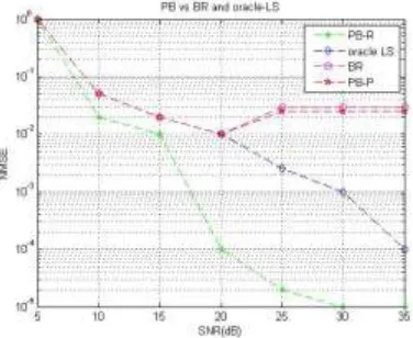
We have simulated a MIMO-OFDM system with a 10 X 10 receive antenna grid. Also we have chosen pilot carrier P randomly and the number of subcarrier taken N=256 we have used 4-QAM modulation and the Gaussian noise statistics are adjusted according to the desired SNR. Channels of scarcity 3 and varying length L are generated using MATLAB. No hardware is made everything is simulated on MATLAB. All results were averaged over 10 trials. We conducted three different experiments.
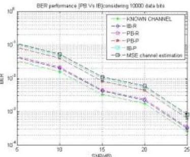
Impact Factor: 4.015
Fig. 2 BER Performance of PB,IB,MMSE
VI.
CONCLUSION
We have proposed and implemented various channel estimation methods for massive MIMO. We have used modified version of SABMP to exploit the sparse common support property and share information in a step by step manner to perform channel recovery. We have also compare with MMSE and showed the best method as the performance is concerned. The approach results in lower communication and computational complexity. Simulation results show superiority over other methods.
REFERENCES
1. W. Bajwa, A. Sayeed, and R. Nowak, “Sparse multipath channels: Modeling and estimation,” in Proc. Digital Signal Processing Workshop and IEEE Signal Processing Education Workshop (DSP/SPE), 2009, pp. 320– 325.
2. H. Minn and V. Bhargava, “An investigation into time-domain approach for OFDM channel estimation,” IEEE Trans. Broadcast., pp. 240–248, 2000.
3. S.-S. Sadough, M. Ichir, P. Duhamel, and E. affrot, “Waveletbased semiblind channel estimation for ultrawideband OFDM systems,” IEEE Trans. Veh. Technol., pp. 1302–1314, 2009.
4. H. Holma and A. Toskala, LTE Advanced: 3GPP Solution for IMT-Advanced. Wiley, 2012.
5. G. J. Foschini, “Layered space-time architecture for wireless communication in a fading environment when using multiple antennas,” Bell Labs Technical Journal, vol. 1, no. 2, pp. 41–59, 1996.
6. P.W.Wolniansky, G. J. Foschini, G. D. Golden, and R. A. Valenzuela, “V-BLAST: an architecture for realizing very high data rates over the rich-scattering wireless channel,” in URSI ISSSE’98, Pisa, Italy, Oct. 1998, pp. 295–300.
7. V. Tarokh, N. Seshadri, and A. R. Calderbank, “Space-time codes for high data rate wireless communication: performance criterion and code construction,” IEEE Trans. Inf. Theory, vol. 44, no. 2, pp. 744–765, Mar. 1998.
8. H. Schoeneich and P. A. Hoeher, “Iterative pilot-layer aided channel estimation with emphasis on interleave-division multiple access systems,” EURASIP Journal on Applied Signal Processing, vol. 2006, pp. 1–15, 2006.
9. T. Zemen, C. Mecklenbrauker, J.Wehinger, and R. Muller, “Iterative joint time-variant channel estimation and multi-user detection for MC-CDMA,” IEEE Transactions on Wireless Communications, vol. 5, pp. 1469–1478, Jun. 2006.
11. S. Suyama, L. Zhang, H. Suzuki, and K. Fukawa, “Performance of iterative multiuser detection with channel estimation for MC-IDMA and comparison with chip-interleaved MC-CDMA,” in Proc. IEEE Global Communications Conference, pp. 1–5, 2008.
12. A. Mukherjee and H. Kwon, “Multicarrier interleave-division multipleaccess systems with adaptive pilot-based user interleavers,” in Proc. IEEE Vehicular Technology Conference, pp. 1–5, 2009.
13. Q. Guo, L. Ping, and D. Huang, “A low-complexity iterative channel estimation and detection technique for doubly selective channels,” IEEE Transactions on Wireless Communications, vol. 8, pp. 4340 –4349, Aug. 2009.