MCs Detection with Combined Image Features and Twin Support Vector Machines

MCs Detection with Combined Image Features

and Twin Support Vector Machines

Xinsheng Zhang

VIPSL, School of Electronic Engineering, Xidian University, Xi’an China School of Management, Xi’an University of Arch. & Tech., Xi’an, China

Email: [email protected]

Xinbo Gao and Ying Wang

VIPSL, School of Electronic Engineering, Xidian University, Xi’an China Email: {xbgao, wying}@lab202.xidian.edu.cn

Abstract—Breast cancer is a common form of cancer diagnosed in women. Clustered microcalcifications(MCs) in mammograms is one of the important early sign. Their accurate detection is a key problem in computer aided detection (CDAe). In this paper, a novel approach based on the recently developed machine learning technique - twin support vector machines (TWSVM) to detect MCs in mammograms. The ground truth of MCs in mammograms is assumed to be known as a priori. First each MCs is preprocessed by using a simple artifact removal filter and a high-pass filter. Then the combined image feature extractors are employed to extract 164 image features. In the combined feature domain, the MCs detection procedure is formulated as a supervised learning and classification problem, and the trained TWSVM is used as a classifier to make decision for the presence of MCs or not. A large number of experiments were carried out to evaluate and compare the performance of the proposed MCs detection algorithm. Experimental results show that the proposed TWSVM classifier is more advantageous for real-time processing of MCs in mammograms.

Index Terms—mammogram, support vector machine, twin support vector machine, microcalcification, ROC curves

I. INTRODUCTION

Breast cancer continues to be a significant public health problem in the world. Mammography is, at present, one of the most effective methods for early detection of breast cancer. One of the important early signs of breast cancer is the appearance of microcalcification clusters (MCs) in mammogram, which appear in 30%-50% of mammogramphically diagnosed cases.

Because of the importance in early breast cancer diagnosis, accurate detection of MCs has become an important problem. Up till now, a number of different approaches have been applied to the detection of MCs. Concerning image segmentation and specification of regions of interest(ROI), several methods have been reviewed [1]. In the past decade, the most work reported in the literature employed neural networks for MCs

characterization [2-6]. With the rise and development of SVM, various SVMs are employed to classify the ROIs [7]. SVM emerged from research in statistical learning theory on how to regulate the trade-off between statistical structural complexity and empirical risk. One of the most popular SVM classifiers is the maximum margin one that attempts to reduce generalization error by maximizing the margin between two disjoint half planes. The resulting optimization task involves the minimization of a convex quadratic objective function subject to linear inequality constraints. While the SVM approach achieves a good performance, the computational complexity of the SVM classifier may prove to be burdensome in real-time or near real-time applications because the solution of the convex optimization problem. Recently Jayadeva et al. [8] proposed a nonparallel plane classifiers for binary data classification, termed as twin support vector machine(TWSVM). It aims at generating two nonparallel planes such that each plane is closer to one of the two classes and is as far as possible from the other. TWSVM solves a pair of quadratic programming problems (QPPs), whereas, in SVM, a single QPP. The two QPPs have a smaller size than the one larger QPP, which makes TWSVM work faster than the standard SVM. It can reduce the optimize process of the solution.

In this work, to improve the performance of the available MCs detection algorithms, we propose to improve the computational efficiency of the pervious approaches by using an alternative, recently developed machine learning technique -- twin support vector machine (TWSVM) for MCs detection to distinguish the MCs from the other ROIs. The advantage of this approach is that the TWSVM classifier can yield a decision function that is much faster than the SVM while maintaining its detection accuracy. The classifier is first trained by the real mammograms from DDSM. Then it is used to detect other ROIs.

and validation and another for test. Compared to several other existing methods, the proposed approach yields superior performance when evaluated using receiver operating characteristic (ROC) curves. It could work 4 times faster than SVM in training stage and achieved the best average sensitivity as high as 93.85% with respect to 5.31% false positive rate and Az=0.9677 in each testing phase.

The rest of the paper is organized as follows: Feature extraction methods are introduced in Section I. A brief review of the theory of TWSVM learning for classification is provided in Section II. The proposed MCs detection algorithm based on TWSVM is formulated in Section III. An evaluation study of the proposed approach is described in Section IV, and the experimental results are given in Section V. Finally, conclusions are drawn in Section VI.

II. COMBINED FEATURES EXTRACTION

The research methodology uses a novel ensemble algorithm with relevance feedback proposed in this paper, for combining a set of features from a number of existing features and detection MCs. As we know, feature extraction is a very important part for the classification. To get the best feature or combination of features and get the high classification rate for microcalcification clusters classification is one of main aims of the proposed research. In our task, a set of 164 features, shown in Table I, is calculated for each suspicious area (ROI) from the textural, spatial and transform domains in our research.

TABLEI COMBINED DIFFERENT KIND OF IMAGE FEATURES USED IN OUR EXPERIMENTS.

Feature groups Type #No.

Histogram based texture features

Mean 1 Standard deviation 2

Smoothness 3 Third moment 4 Uniformity 5 Entropy 6

Multi-scale histogram features

Histograms with different number of bins 3,5,7,9

7~30(total 24)

Zernike Moments

Features[9] Zernike Moments

31~66 (total 36, D=10)

Combined first 4 moments features

Combined moments

feature 67~114 (total 48)

Tamura texture signatures Tamura features 115~120 (total 6) Chebyshev transform

histogram feature [10]

Chebyshev

histogram 121~152 (total 32) Radon Transform Features Radon features 153~164 (total 12)

Before training the classifier, we use the feature extractor discussed in Table I to extract MCs features in the feature domain. The 164 features of each block are extracted as follows:

(1) Intensity histogram based texture feature

A frequently used approach for texture analysis is based on statistical properties of the intensity histogram. One class of such measures is based on statistical

moments. The expression for the nth moment about the mean is given by

1

0( ) ( )

L _n

n i zi m p zi

P

¦

(1) whereziis a random variable indicating intensity, p z( )is

the histogram of the intensity levels in a region, Lis the number of possible intensity levels, and

1 0 ( )

L

i i

i

m

¦

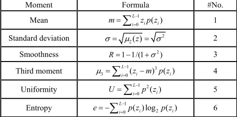
z p z (2) is the mean(average)intensity. Table 2 lists the descriptors used in our experiments based on statistical moments and also on uniformity and entropy.

TABLEII DESCRIPTORS OF THE TEXTURE BASED ON THE INTENSITY HISTOGRAM OF A REGION.

Moment Formula #No.

Mean m Li₀1z p zi ( )i

¦

1

Standard deviation 2

2( )z

V P V 2

Smoothness 2

1 1/(1 )

R V 3 Third moment 3 01( )3 ( )

L

i i i z m p z

P

_¦

4

Uniformity 1 2

0 ( )

L i i

U

_¦

p z 5

Entropy 01 ( ) log2 ( )

L

i i i

e

_¦

p z p z 6

(2) Multiscale intensity histograms

We compute signatures based on "multi-scale histograms" idea. Idea of multi-scale histogram comes from the belief of a unique representation of an image through infinite series of histograms with sequentially increasing number of bins. Here we used 4 histograms with number of bins being 3,5,7,9 to calculate the image feature, so we get a 1*24 row vectors.

(3) Zernike moments

We use derived moments based on alternative complex polynomial functions, know as Zernike polynomials[9]. They form a complete orthogonal set over the interior of the unit circle _x2_y2 _{1 and are defined as}

2 2₁

( 1) / ( , ) ( , ) ,

pq

x y

Z p S

_³

_d f x y V U T dxdy (3) ( , ) ( , ) ( ) exp( ),

pq pq pq

V x y V U T R U jqT (4)

( ) / 2 2

0

( 1) [( )!]

( ) ,

! ! !

2 2

p q s p s

pq s

p s R

p q p q

s s s

U U

§ · § ·

¨ ¸ ¨ ¸

© ¹ © ¹

¦

(5)

where p is a nonnegative integer, q is an integer subject to the constraint p q even and q d p, 2 2

x y

U

is the radius from ( , )x y to the image centroid,

1

tan ( / )y x

T

is the angle between U and x-axis. The Zernike momentZ_pqis orderp with repetition q. For a digital image, the respective Zernike moments are computed as

2 2

( 1) / ( , ) ( , ) , 1,

pq i i

i

(4) Combined first four moment features

Signatures on the basis of first four moments (also known as mean, std, skewness, kurtosis) for data generated by vertical, horizontal, diagonal and alternative diagonal 'combs'. Each column of the comb results in 4 scalars [mean, std, skewness, kurtosis], we have as many of those [...] as 20. So, 20 go to a 3-bin histogram, producing 1x48 vectors.

(5) Tamura texture signatures

Tamura et al. took the approach of devising texture features that correspond to human visual perception [10]. Six textural features: coarseness, contrast, directionality, line-likeness, regularity and roughness, are defined for the image feature for object recognition.

(6) Transform domains feature

We computes signatures (32 bins histogram) from coefficients of 2D Chebyshev transform (10th order is used in our experiments). Also we used signatures based on the Radon transform as a kind of image features. Radon transform is the projection of the image intensity along a radial line (at a specified orientation angle), total 4 orientations are taken. Transformation n/2 vectors (for each rotation), go through 3-bin histogram and convolve into 1x12 vectors.

III. TWINSUPPORT VECTOR MACHINES

In this paper, MCs detection is formulated as a binary (+1, -1) classification problem. At each location in a mammogram, the trained TWSVM classifier is applied to determine where a MCs object is present or not. We defined n

R



x as a pattern to be classified, and y as its class label (i.e., y{r1} ). In addition, let {(xi,yi),i 1,2,...,m} denote a given set of m training

examples. And meanwhile we define m row vectors Ai(i 1,2,...m) in the n dimensional real

space n

R , where Ai (Ai1,Ai2,...,Ain) and then T i i A x . Here data points belonging to classes 1 and -1 are represented by matrices A and B. Let the number of patterns in class 1 and -1 be given by m1 and m2.

Therefore, the sizes of matrices A and B are (m1un)

and (m2un), respectively.

A. Linear TWSVM Classifier

Twin support vector machine (TWSVM) [8] obtains nonparallel planes around which the data points of the corresponding class get clustered. Each of the two quadratic programming problems in the TWSVM pair has the formulation of a typical SVM, except that not all patterns appear with constrains of either problem at the same time.

The TWSVM classifier is obtained by solving the following pair of quadratic programming problems

and b

c b

b T T

, 0 , ) ( -s.t. ) ( ) ( 2 1 min ) TWSVM1 ( 2 (1) 2 (1) 2 1 ) 1 ( 1 ) 1 ( ) 1 ( 1 ) 1 ( , b , (1) (1) t t q e q e Bw q e e Aw e Aw q

w (7)

, 0 , ) ( s.t. ) ( ) ( 2 1 min ) TWSVM2 ( 1 (2) 1 (2) 1 2 ) 2 ( 2 ) 2 ( ) 2 ( 2 ) 2 ( , b , (2) (2) t t q e q e Aw q e e Bw e Bw q w b c b

b T T

(8)

where c1,c2!0 are parameters and e1 and e2 are

vectors of ones of appropriate dimensions.

This algorithm aims to find two optimal hyperplanes, one for each class, and classifiers points according to which hyperplane a given point is closest to. The first term in the objective function of (7) or (8) is the sum of squared distances from the hyperplane to points of one class. Therefore, minimizing it tends to keep the hyperplane close to points of one class (say class 1). The constraints require the hyperplane to be at a distance of at least 1 from points of the other class (say class -1); a set of error variables is used to measure the error wherever the hyperplane is closer than this minimum distance of 1. The second term of the objective function minimizes the sum of error variables, thus attempting to minimize misclassification due to points belonging to class -1.

B. Kernel TWSVM Classifier

The linear TWSVM can be easily extended to a nonlinear classifier by first using a nonlinear operator

) (˜

) to map the input pattern x into a higher dimensional space Ǿ , where the function K(˜,˜) is defined as

). ( ) ( ) ,

(x y {)T x) y

K (9) And the kernel-generated surfaces instead of planes are defined as follows:

, 0 ) , ( and , 0 ) ,

( (1) (1) (2) (2)

b K C b

K T T T T

u x u C x (10)

where T [ B]T,

A

C and K is an appropriately chosen kernel, such as polynomial kernel, RBF kernel etc.. Compared with the above arguments, the optimization problem of Kernel TWSVM (KTWSVM1, KTWSVM2) is defined as:

(1) (1)

(1) (1)

1 1 2

, b ,

(1) (1)

2 2

1

(KTWSVM1) min ( , ) 2

s.t. ( , ) , 0,

T T

T

K b c

K B b

t t

u q A C u e e q

C u e q e q

(11

)

(2) (2)

(2) (2)

2 2 1

, b ,

(2) (2)

1 1

1

(KTWSVM2) min ( , ) 2

s.t. ( , ) , 0,

T T

T

K u b c K A u b

t t

u q

B C e e q

C e q e q

(12) where c1!0, and c2!0 are tuned parameters.

In the paper, we use the popular polynomial kernels and the RBF kernels, which are known to satisfy the Mercer’s condition. They are defined as follows,

1) Polynomial kernel:

, ) 1 ( ) ,

( T p

K x y x y

(13) where p!0is a constant that defines as the kernel order.

2) RBF kernel:

, 2 exp ) , ( ₂ 2 ¸ ¸ ¹ · ¨ ¨ © § V y x y x

where V !0is a constant that defined as the kernel width.

IV. MCSDETECTION WITHTWSVM

For a given digital mammography image, we consider the MCs detection process as the following steps:

y Step 1. Preprocess the mammography image by removing the artifacts, suppressing the inhomogeneity of the background and enhancing the microcalcifications.

y Step 2. At each pixel location in the image, extract a Amum small window to describe its

surrounding image feature.

y Step 3. Apply feature extraction methods to get the combined feature vector x.

y Step 4. Use the trained TWSVM classifier to make decision whether x belongs to MCs class (+1) or not (-1).

A. Mammogram Preprocessing

First, a simple film-artifact removal filter is applied to remove the film-artifacts from mammography image. There are small emulsion continuity faults on the X-ray mammogram films, which look like microcalcifications. These artifacts are usually sharply defined and brighter than the microcalcifications, and the size of the artifacts is within 5u5 pixels in our experiments.

Let us consider two windows centered on a current pixel (x,y) . R1 is the inner region and R₂ is the

surrounding region. If the difference between the pixel value at the current position (x,y), I(x,y), and the mean value of the surrounding region A(x, y) is larger than a threshold value, T , then the pixel value of current position is substituted by the mean value of the surrounding region R2. The output of the filmartifacts

removal filtering, I1(x,y), is defined as

¯ ®

­ !

. ),

, (

)] , ( ) , ( [ ), , ( ) , (

1

otherwise y

x I

T y x A y x I if y x A y x

I (15)

In (15), the threshold value, T , is empirically selected from many digitized mammograms so that the film-artifacts can be removed and the microcalcifications can be preserved.

After the artifacts were removed, our task is to suppress the mammogram background. A high-pass filter is designed to preprocess each mammogram before extracting samples. With the Gaussian filter,

2 2 2

( , ) exp( ( ) /(2 ))

f x y x y V , we use a mum window size Gaussian filter where 4 21

V

m , experimentally in the study V 2 . The output of high-pass filter is denoted by I2(x,y) I1(x,y)f(x,y)I1(x,y), where is

linear convolution.

B. Input Patterns for MCs detection

After the mammogram preprocessing stage, we extract combined image features from Amum as a feature vector

x. Amum is a small window of mum pixels centered at a

location that we concerned in a mammogram image. The choice of m should be large enough to include the MCs (in our experiment, we take m=115). The task of the TWSVM classifier is to decide whether the input window

m m

A_u at each location is a MCs pattern (y 1) or not (y 1).

C. Training Data Set Preparation

The procedure for extracting training data from the training mammograms is given as follows. For each MCs location in a training mammogram set, a window of

m

mu image pixels centered at its center of mass is extracted; the area is denoted by Aimum, with respect to xi

after subspace feature extraction, and then xi is treated as

an input pattern for the positive sample (yi 1). The

negative samples are collected (yi 1) similarly, except

that their locations are randomly selected from the non MCs locations in the training mammograms. In the procedure, no window in the training set is allowed to overlap with any other training window.

D. TWSVM training and Parameter Selection

After the positive and negative training examples are gathered, some parameters should be initialized first, such as the type of kernel function, its associated parameter, and the regularization parameter c1 and c2 in the

structural risk function. To optimize these parameters, we applied m -fold cross validation method to get the optimal parameters.

Once the best parametric setting (i.e., the type of the kernel function and its associated parameter) is determined, the TWSVM classifier is retrained using all the available samples in the training set to obtain the final form of the decision function. The resulting classifier will be used to detect the MCs in mammogram.

V DATABASE AND PERFORMANCE EVALUATION

A. Mammographic Database

In this research Digital Database for Screening Mammography (DDSM) from University of South Florida is used for experiments. The optical density range of the scanner for the database was 0-3.6. The 12bits digitizer was calibrated so that the gray values were linearly and inversely proportional to the optical density. In DDSM database, the boundaries for the suspicious regions are derived from markings made on the film by at least two experienced radiologists.

B. Performance Evaluation Methods

correction of classification accuracy may be misleading. Unfortunately, in real-life problems, these assumptions are not always true. Consequently, the performance of such systems is best described in terms of their sensitivity and specificity quantifying their performance related to false positive and false negative instances. These metrics are based on the consideration that a test point always falls into one of the following four categories:

y False Positive (FP): if the system labels a negative point as positive;

y False Negative (FN): if the system labels a positive point as negative;

y True Positive (TP): if the system correctly predicts the label;

y True Negative (TN): if the system correctly predicts the label.

The sensitivity or true positive of a learning machine, which is also called recall, is defined as the ration between the number of true positive predictions TP and the number of positive instances in the test set. It is defined as follows:

/( ).

Sensitivity TP TPFN (10) While the specificity or true negative rate is defined as the ratio between the number of true negative predictions TN and the number of negative instance in the test set. It is defined as

/( )

Specificity TN TNFP (11) The overall accuracy is the ratio between the total number of correctly classified instances and the test set size. It is defined as

/

r

OverallAccuracy N N (12) where Nr TPTN is the number of correctly

classified samples during the test run and

N TP TN FPFN is the complete number of test samples.

Another important measure is the area under curve (Az) wherein the curve is the receiver operating characteristic (ROC) curve [11]. ROC curve is a plotting of true positive as a function of false positive. Higher ROC, approaching the perfection at the upper left hand corner, would indicate greater discrimination capacity.

VI EXPERIMENTAL RESULTS

A. Combined Feature Extraction

The data in the training (and validation), test, and validation sets were randomly selected from the training set. Each selected sample was covered by a 115x115 window whose center coincided with the center of mass of the suspected MCs. The blocks included 2231 with true MCs and 8364 with normal tissue.

Before training the classifier, we first use the feature extraction algorithm to extract MCs feature in combined feature domain. The 164-dimension feature vector will be calculated for each image block. When we get the image feature vector, feature normalization program should be user for normalizing the features to be real numbers in the range of [0, 1]. The normalization is accomplished by the following step: (a) change all the features to be positive

by adding the magnitude of the largest minus value of this feature times 1.012, (b) divided by the maximum value of the same feature. The normalized features are used as the inputs of the proposed ensemble learning algorithm for training and classification.

B. TWSVM Training and Model Selection

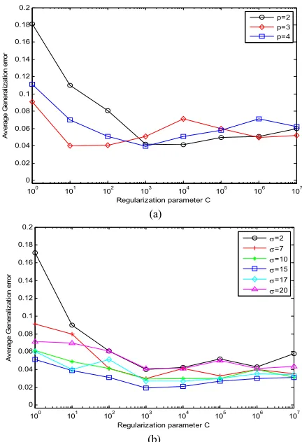
For model selection, the TWSVM classifier is first trained by using the 10-fold cross-validation procedure with different model and parametric settings. In our training stage, we used generalization error, which was defined as the total number of incorrectly classified examples divided by the total number of samples classified, as a metric to measure the trained classifier. Generalization error was computed using only the samples used during training. For the sake of convenient, the parametric values of c1 and c2in our experiment are

set to be equal (i.e. c1 c2). In Fig. 1(a), we summarize

the results for trained TWSVM classifier with a polynomial kernel. The estimated generalization error is plotted versus the regularization parameters c1 and c2 for

kernel orderp 2, p 3 andp 4. Similarly, Fig. 4(b) summarizes the results with RBF kernel. Here, the generalization error is plotted for different values of the width V (2, 7, 10, 15, 17, 20).

100 101 102 103 104 105 106 107 0

0.02 0.04 0.06 0.08 0.1 0.12 0.14 0.16 0.18 0.2

Regularization parameter C

A

v

er

ag

e G

ener

al

iz

at

ion

er

ro

r

p=2 p=3 p=4

(a)

100 101 102 103 104 105 106 107 0

0.02 0.04 0.06 0.08 0.1 0.12 0.14 0.16 0.18 0.2

Regularization parameter C

A

v

e

rage G

e

ner

al

iz

at

io

n

er

ro

r

V=2

V=7

V=10

V=15

V=17

V=20

(b)

Fig. 1 Plot of average generalization error rate versus regularization parameter C (c1 c2) achieved by training TWSVM using (a) a

For the polynomial kernel, it is found that the smallest generalization error is get when p 3 and c1 and c2 are

between 100 and 1000. A similar error level was also achieved by the RBF kernel over a wide range of parameter settings (e.g., V 15 and c1,c2[100,1000]).

These results indicate that the performance of the TWSVM classifier is not very sensitive to the model parameters. Indeed, essentially similar performance was achieved when V was varied from 10 to 20.

Having determined that the TWSVM results do not vary significantly over a wide range of parameter settings, next we will focus for the remainder of the paper on a particular, representative configuration of the TWSVM classifier, having a RBF kernel with V 15

and c1 c2 1000.

For comparison, we also trained the SVM classifier using the same training procedure as for the TWSVM. The best error level (3.1%) was achieved when an RBF kernel with V 15and the regularization parameter c

was set to 10. Similar to TWSVM, the SVM classifier was retrained using these tuned parameters with all the samples in the training set.

For the TWSVM classifier, the number of SVs (on the two nonparallel planes) was 83 (500 positive and 500 negative samples); for SVM the number of SVs (on the two parallel planes) was 285 (500 positive and 500 negative samples). We can see that the TWSVM classifier is much effective than the traditional SVM method.

C. Performance Evaluation Results

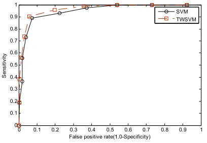
The trained classifiers are evaluated using all the mammograms in the test subset. The test results are summarized by using ROC curves in Fig.2 for TWSVM. For comparison, ROC curve is also show for the traditional SVM classifier with the same inputs. Average experimental results of TWSVM and SVM classifier are shown in Table I.

TABLE III.

EXPERIMENTAL RESULTS OF TWSVM AND SVM CLASSIFIER.

Method Sensitivity Specificity Az

SVM 0.9201 0.9237 0.9586

TWSVM 0.9385 0.9469 0.9706

From the Fig. 2, it can be shown that, the TWSVM classifier has a higher detection accuracy rate compared to SVM classifier. By using the same extracted feature, compared with SVM, TWSVM has a better detection rate and run about 4 times faster than the SVM when we train the classifier. In particular, the TWSVM classifier achieved a sensitivity of approximately 93.85% with respect to 5.31% false positive rate and Az=0.9706. With the same training data set and test data set, the SVM classifier achieved a sensitivity of 92.01% , 7.63% false positive rate and Az=0.9586.

D. Experimental Execution Times Analysis

Finally, we show in Table IV the computation times for the different methods (implemented with MATLAB on

an Intel Core 2 CPU 1.86 GHz, DDR2 1.99GB PC). The training time is the average amount of time taken during each round of training in the 10-fold cross validation procedure during the training phase; the test time is the average amount of time taken by the trained classifier for classifying each image during the testing phase. Compared to SVM, the TWSVM classifier has reduced the detection time to about 1/4. Note that such a dramatic saving in computation time is achieved without sacrificing the best detection. This is because TWSVM solves a pair of quadratic programming problems (QPPs), whereas, in SVM, a single QPP. The two QPPs have a smaller size than the one larger QPP, which makes TWSVM work faster than the standard SVM.

0 0.1 0.2 0.3 0.4 0.5 0.6 0.7 0.8 0.9 1 0

0.1 0.2 0.3 0.4 0.5 0.6 0.7 0.8 0.9 1

False positive rate(1.0-Specificity)

S

e

n

s

it

iv

it

y

SVM TWSVM

Fig. 2. Roc curves MCS detection by using SVM and TWSVM classifier, where Az (SVM)=0.9586 and Az (TWSVM)=0.9706.

TABLE IV.

THECOMPUTATION TIME FOR TWSVM AND SVM CLASSIFIERS. THE

TRAINING TIME IS AVERAGE AMOUNT OF TIME TAKEN DURING EACH

ROUND OF TRAINING IN THE 10-FOLD CROSS VALIDATION PROCEDURE, AND THE TESTING TIME IS THE AVERAGE AMOUNT OF TIME TAKEN BY

THETRAINED CLASSIFIER FOR CLASSIFYING EACHIMAGE DURING THE

TESTING PHASE

SVM TWSVM

Training time(s) 4.9726 1.3127

Testing time(s) 0.3515 0.2801

VII. CONCLUSION

ACKNOWLEDGMENT

This work presented in our paper is supported by the National Natural Science Foundation of China (No. 60771068), the Natural Science Basic Research Plan in Shaanxi Province of China (No. 2007F248) and the Youth Scientific Research Foundation in Xi’an Univ. of Arc. & Tech. (No. QN0738). The authors are grateful for the anonymous reviewers who made constructive comments.

REFERENCES

[1] H. D. Cheng, X. Cai, X. Chen et al., “Computer-aided detection and classification of microcalcifications in mammograms: a survey,” Pattern Recognition, vol. 36, no. 12, pp. 2967-2991, 2003.

[2] S. Halkiotis, T. Botsis, and M. Rangoussi, “Automatic detection of clustered microcalcifications in digital mammograms using mathematical morphology and neural networks,” Signal Processing, vol. 87, no. 7, pp. 1559-1568, 2007.

[3] R. R. Hernandez-Cisneros, and H. Terashima-Marin, "Evolutionary Neural Networks Applied To The Classification Of Microcalcification Clusters In Digital Mammograms." pp. 2459-2466.

[4] A. Papadopoulos, D. I. Fotiadis, and A. Likas, “Characterization of clustered microcalcifications in digitized mammograms using neural networks and support vector machines,” Artificial Intelligence in Medicine, vol. 34, no. 2, pp. 141-150, 2005.

[5] L. Bocchi, G. Coppini, J. Nori et al., “Detection of single and clustered microcalcifications in mammograms using fractals models and neural networks,” Medical Engineering & Physics, vol. 26, no. 4, pp. 303-312, 2004. [6] Y. Songyang, and G. Ling, “A CAD system for the

automatic detection of clustered microcalcifications in digitized mammogram films,” IEEE Trans. Med. Imag.,

vol. 19, no. 2, pp. 115-26, 2000.

[7] I. El-Naqa, Y. Yongyi, M. N. Wernick et al., “A support vector machine approach for detection of microcalcifications,” IEEE Trans. Med. Imag., vol. 21, no. 12, pp. 1552-1563, 2002.

[8] Jayadeva, R. Khemchandani, and S. Chandra, “Twin Support Vector Machines for Pattern Classification,” IEEE Trans. Pattern Anal. Mach. Intell., vol. 29, no. 5, pp. 905-910, 2007.

[9] L. Tsong-Wuu, and C. Yun-Feng, "A comparative study of Zernike moments." pp. 516-519.

[10] M. S. Tamura H., Yamawaki T., “Texture features corresponsing to visual perception,” Systems, Man and Cybernetics, IEEE Transactions. on, vol. 1, no. 8, pp. 460-472, 1978

[11] J. B. Tilbury, W. J. Van Eetvelt, J. M. Garibaldi et al., “Receiver operating characteristic analysis for intelligent medical systems-a new approach for finding confidence intervals,” IEEE Trans. Biomed. Eng., vol. 47, no. 7, pp. 952-963, 2000.

Xinsheng Zhang is presently pursuing his PhD degree in school of Electronic Engineering, Xidian University. He received his M.S. Degree and the B.S. degree in system engineering from Xi’an University of Architecture & Technology, China, in 2004 and 2001, respectively.

His research interests include image processing and machine learning.

Xinbo Gao received the B.S. degree in electronic engineering, and the M.S. and Ph.D. degrees in signal and information processing from Xidian University, Xi’an, in 1994, 1997, and 1999, respectively.From 1997 to `1998, he was with the computer Games Research Institute, Shizuoka University, as a Research Fellow. From 2000 to 2001, he also worked at the multimedia Laboratory, Chinese University of Hong Kong, Hong Kong, as a Research Associate. Since 2003, he has been a full Professor in the School of Electronic Engineering at Xidian University, Xi'an, China, and the Director of Video/Image Processing System Laboratory (VIPSL).