ISSN (e): 2250-3021, ISSN (p): 2278-8719
Vol. 05, Issue 02 (February. 2015), ||V1|| PP 13-26
M/M/C Bulk Arrival And Bulk Service Queue With Randomly
Varying Environment
Sandhya.
𝑅
1, Sundar.
𝑉
2, Rama.G
3, Ramshankar.R
4, Ramanarayanan.R
51
Independent Researcher MSPM, School of Business, George Washington University, Washington .D.C, USA
2
Senior Testing Engineer, ANSYS Inc., 2600, Drive, Canonsburg, PA 15317, USA
3
Independent Researcher B. Tech, Vellore Institute of Technology, Vellore, India 4
Independent Researcher MS9EC0, University of Massachusetts, Amherst, MA, USA
5
Professor of Mathematics, (Retired), Veltech University, Chennai
Abstract: - This paper studies two stochastic bulk arrival and bulk service C server queues (A) and (B) with k varying environments. The arrival and service times are exponential random variables and their parameters change when the environment changes. The system has infinite storing capacity and the arrival and service sizes are finite valued random variables. Matrix partitioning method is used to study the models. In Model (A) the maximum of the arrival sizes M in all the environments is greater than the maximum of the service sizes N in all the environments, (M > N), and the infinitesimal generator is partitioned as blocks of k times the maximum of the arrival sizes for analysis. In Model (B) the maximum of the arrival sizes M in all the environments is less than the maximum of the service sizes N in all the environments, (M < N), where the generator is partitioned using blocks of k times the maximum of the service sizes. Five different cases associated with C, M and N due to partitions are treated. They are namely, (A1) M >N ≥ C, (A2) M >C >N (A3) C >M >N, which come up in Model (A); (B1) N ≥ C and (B2) C >N, which come up in Model (B) respectively. For the cases when C ≤ M or N Matrix Geometric results are obtained and for the cases when C > both M and N Modified Matrix Geometric results are presented. The basic system generator is seen as a block circulant matrix in all the cases. The stationary queue length probabilities, its expected values, its variances and probabilities of empty queue levels are derived for the models using Matrix Methods. Numerical examples are presented for illustration.
Keywords:Block Circulant, Bulk Arrival, Bulk Service, C servers, Infinitesimal Generator, Matrix methods.
I. INTRODUCTION
are very common. Manufactured products arrive in bulk sizes and several bulk sizes of products are sold in markets. Recently M/M/1 queue system with disaster has been studied by Noam Paz and Uri Yechali [9] but random arrival size or random service size with varying environments is not studied. Usually the partitions of the bulk arrival models have M/G/1 upper-Heisenberg block matrix structure with zeros below the first sub diagonal. The decomposition of a Toeplitz sub matrix of the infinitesimal generator is required to find the stationary probability vector. Matrix geometric structures have not been noted so far as mentioned by William J. Stewart [10]. But in this paper the partitioning of the matrix is carried out in a way that the stationary probability vectors have a Matrix Geometric solution or a Modified Matrix Geometric solution for infinite capacity C server bulk arrival and bulk service queues with randomly varying environments.
Two models (A) and (B) on M/M/C bulk queue systems under k varying environments with infinite storage space for customers are studied here using the block partitioning method. In the models considered here, the maximum arrival sizes and the maximum service sizes may be different for different environments. Model (A) presents the case when M, the maximum of all the maximum arrival sizes in all the environments is bigger than N, the maximum of all the maximum sale sizes in all the environments. In Model (B), its dual, N is bigger than M, is treated. In general in Queue models, the state space of the system has the first co-ordinate indicating the number of customers in the system but here the customers in the system are grouped and considered as members of M sized blocks of customers (when M >N) or N sized blocks of customers (when N > M) for finding the rate matrix. Using the maximum of the bulk arrival size or maximum of the bulk service size and grouping the customers as members of the blocks for the partitioning the matrix of the infinitesimal generator along with the environment state is a new approach in this area. In [1], Rama Ganesan, Ramshankar and Ramanarayanan for single server M/M/1 bulk queue, have noticed two cases namely M >N and N >M but in this paper because a multi server system is of interest five cases are noticed. Model (A) gives three cases namely (A1) M > N ≥ C, (A2) M > C > N and (A3) C > M > N and Model (B) gives two cases namely (B1) N ≥ C, and (B2) C > N. The case M=N with various C values can be treated using Model (A) or Model (B). For the cases when C ≤ M or N, Matrix Geometric results are obtained and for the cases when C > both M and N, Modified Matrix Geometric results are presented. The matrices appearing as the basic system generators in these models due to block partitions are seen as block circulant matrices. The stationary probability of the number of customers waiting for service, the expected queue length, the variance and the probability of empty queue are derived for these models. Numerical cases are presented to illustrate their applications. The paper is organized in the following manner. In section II and section III the M/M/C bulk arrival and bulk service queues with randomly varying environment in which maximum arrival size M is greater than maximum service size N and the maximum arrival size is M less than the maximum service size N are studied respectively with their sub
cases. In section IV numerical cases are presented.
II. MODEL (A). MAXIMUM ARRIVAL SIZE M IS GREATER THAN MAXIMUM
SERVICE SIZE N
2.1Assumptions for M > N.
i) There are k environments. The environment changes as per changes in a continuous time Markov chain with infinitesimal generator 𝒬1 of order k with stationary probability vector ϕ. ii) Customers arrive in different bulk sizes for service. The time between consecutive bulk arrivals of customers has exponential distribution with parameter𝜆𝑖, in the environment i for 1 ≤ i ≤ k. At each bulk arrival in the
environment i, 𝜒𝑖 customers arrive with probability P (𝜒𝑖= j) = 𝑝𝑗𝑖 for 1 ≤ j ≤ 𝑀𝑖 and 𝑝𝑗𝑖 𝑀𝑖
𝑗 =1 =1 for 1 ≤ i ≤ k.
iii) Customers are served in batches of different bulk sizes. There are s servers to serve when s customers are present in the system for 1≤ s ≤ C. When C or more than C customers are present in the system the number of servers to serve customers is C. In the environment i for1 ≤ i ≤ k, the time between consecutive bulk services has exponential distribution with parameter s𝜇𝑖 when s customers are in the system for 1≤ s ≤ C and with
parameter C𝜇𝑖 when C or more than C customers are present where 𝜇𝑖 is the parameter of single server
exponential service time distribution. At each service epoch in the environment i, 𝜓𝑖 customers are served with
probability given by P (𝜓𝑖 = j) = 𝑞𝑗𝑖 for 1≤ j ≤ 𝑁𝑖 when more than 𝑁𝑖 customers are waiting for service
where 𝑞𝑗𝑖 𝑁𝑖
for 1≤ j ≤ n-1 and n customers are served with probability 𝑁𝑖 𝑞𝑗𝑖
𝑗 =𝑛 for 1 ≤ i ≤ k.
iv) When the environment changes from i to j, the parameter of time between consecutive bulk arrivals and the service parameter change from (𝜆𝑖 , 𝜇𝑖) 𝑡𝑜 (𝜆𝑗, 𝜇𝑗 ), the bulk arrival size 𝜒𝑖 changes to 𝜒𝑗, the bulk service size 𝜓𝑖changes to 𝜓𝑗 and the maximum arrival size 𝑀𝑖 and the maximum service size 𝑁𝑖 change to 𝑀𝑗 𝑎𝑛𝑑 𝑁𝑗 for
1≤i,j≤k.
v) The maximum of the maximum of arrival sizes M = max1 ≤𝑖 ≤𝑘𝑀𝑖 is greater than the maximum of the
maximum of service sizes N =max1 ≤𝑖 ≤𝑘𝑁𝑖.
2.2 Analysis
There are three sub cases for this model namely (A1) M > N ≥ C, (A2) M > C >N and (A3) C > M >N. Sub Cases (A1) and (A2) admit Matrix Geometric solutions and they are treated in sub section (2.2.1). Modified Matrix Geometric solution is presented for Sub Case (A3) which is studied in sub section (2.2.2). The state of
the system of the continuous time Markov chain X (t) under consideration is presented as follows. X (t) = {(n, j, i): for 0 ≤ j ≤ M-1; 1 ≤ i ≤ k and n ≥ 0}
(1) The chain is in the state (n, j, i) when the number of customers in the system is n M + j, for 0 ≤ j ≤ M-1 and 0 ≤ n < ∞ and the environment is i for 1 ≤ i ≤ k. When the number of customers in the system is r, then r is identified with (n, j) where r on division by M gives n as the quotient and j as the remainder. Let the survivor
probability of the number of arrivals at an arrival epoch and the number of services at a service epoch in the environment i for 1 ≤ i ≤ k be P (𝜒𝑖 > j) = 𝑃𝑗𝑖=1- 𝑝𝑛𝑖
𝑗
𝑛=1 , and 𝑃0𝑖 = 1 for 1 ≤ j ≤ 𝑀𝑖-1 (2)
and P (𝜓𝑖 > j) = 𝑄𝑗𝑖=1- 𝑞𝑛𝑖 𝑗
𝑛=1 , and 𝑄0𝑖 = 1 for 1 ≤ j ≤ 𝑁𝑖-1 (3) 2.2.1 Sub Cases: (A1) M > N ≥ C and (A2) M > C > N
When M > N ≥ C or M > C > N, the M/M/C bulk queue admits matrix geometric solution as follows. The chain X (t) describing them, has the infinitesimal generator 𝑄𝐴,2.1 of infinite order which can be presented in block
partitioned form given below.
𝑄𝐴,2.1 =
𝐵1 𝐴0 0 0 . . . ⋯
𝐴2 𝐴1 𝐴0 0 . . . ⋯
0 𝐴2 𝐴1 𝐴0 0 . . ⋯
0 0 𝐴2 𝐴1 𝐴0 0 . ⋯
0 0 0 𝐴2 𝐴1 𝐴0 0 ⋯
⋮ ⋮ ⋮ ⋮ ⋱ ⋱ ⋱ ⋱
(4)
In (4) the states of the matrices are listed lexicographically as 0,1, 2, 3, … . 𝑛, …. Here the vector 𝑛 is of type 1 x
k M and 𝑛 = ((n, 0, 1),(n, 0, 2)…(n, 0, k),(n, 1, 1),(n, 1, 2)…(n, 1, k)…(n, M-1, 1),(n, M-1, 2)… (n, M-1, k)) for n ≥ 0. The matrices 𝐵1𝑎𝑛𝑑 𝐴1 have negative diagonal elements, they are of order Mk and their
off diagonal elements are non- negative. The matrices 𝐴0, 𝑎𝑛𝑑𝐴2 have nonnegative elements and are of order Mk and they are given below. Let the following be diagonal matrices of order k
𝛬𝑗=diag (𝜆1𝑝𝑗1, 𝜆2𝑝𝑗2, … . , 𝜆𝑘𝑝𝑗𝑘) 𝑓𝑜𝑟 1 ≤ 𝑗 ≤ 𝑀; 𝑈𝑗 = diag 𝜇1𝑞𝑗1, 𝜇2𝑞𝑗2, … . , 𝜇𝑘𝑞𝑗𝑘 𝑓𝑜𝑟 1 ≤ 𝑗 ≤ 𝑁 (5)
𝑉𝑗 = diag 𝜇1𝑄𝑗1, 𝜇2𝑄𝑗2, … . , 𝜇𝑘𝑄𝑗𝑘 𝑓𝑜𝑟 1 ≤ 𝑗 ≤ 𝑁; 𝛬 =diag (𝜆1, 𝜆2, … . , 𝜆𝑘); 𝑈 = diag (𝜇1, 𝜇2, … . , 𝜇𝑘) (6) 𝐿𝑒𝑡 𝒬1′ = 𝒬1− 𝛬 − 𝐶𝑈. (7)
Here 𝒬1 is the infinitesimal generator of the Markov chain of the environment defined earlier
𝐴0=
𝛬𝑀 0 ⋯ 0 0 0
𝛬𝑀−1 𝛬𝑀 ⋯ 0 0 0
𝛬𝑀−2 𝛬𝑀−1 ⋯ 0 0 0
𝛬𝑀−3 𝛬𝑀−2 ⋱ 0 0 0
⋮ ⋮ ⋱ ⋱ ⋮ ⋮
𝛬3 𝛬4 ⋯ 𝛬𝑀 0 0
𝛬2 𝛬3 ⋯ 𝛬𝑀−1 𝛬𝑀 0
𝛬1 𝛬2 ⋯ 𝛬𝑀−2 𝛬𝑀−1 𝛬𝑀
(8)
𝐴2
=
0 ⋯ 0 𝐶𝑈𝑁 𝐶𝑈𝑁−1 ⋯ 𝐶𝑈2 𝐶𝑈1
0 ⋯ 0 0 𝐶𝑈𝑁 ⋯ 𝐶𝑈3 𝐶𝑈2
⋮ ⋮ ⋮ ⋮ ⋮ ⋱ ⋮ ⋮
0 ⋯ 0 0 0 ⋯ 𝐶𝑈𝑁 𝐶𝑈𝑁−1
0 ⋯ 0 0 0 ⋯ 0 𝐶𝑈𝑁
0 ⋯ 0 0 0 ⋯ 0 0
⋮ ⋮ ⋮ ⋮ ⋮ ⋮ ⋮ ⋮
0 ⋯ 0 0 0 ⋯ 0 0
𝐴1=
𝒬1′ 𝛬1 𝛬2 ⋯ 𝛬𝑀−𝑁−2 𝛬𝑀−𝑁−1 𝛬𝑀−𝑁 ⋯ 𝛬𝑀−2 𝛬𝑀−1
𝐶𝑈1 𝒬1′ 𝛬1 ⋯ 𝛬𝑀−𝑁−3 𝛬𝑀−𝑁−2 𝛬𝑀−𝑁−1 ⋯ 𝛬𝑀−3 𝛬𝑀−2
𝐶𝑈2 𝐶𝑈1 𝒬1′ ⋯ 𝛬𝑀−𝑁−4 𝛬𝑀−𝑁−3 𝛬𝑀−𝑁−2 ⋯ 𝛬𝑀−4 𝛬𝑀−3
⋮ ⋮ ⋮ ⋱ ⋮ ⋮ ⋮ ⋱ ⋮ ⋮
𝐶𝑈𝑁 𝐶𝑈𝑁−1 𝐶𝑈𝑁−2 ⋯ 𝒬1′ 𝛬1 𝛬2 ⋯ 𝛬𝑀−𝑁−2 𝛬𝑀−𝑁−1
0 𝐶𝑈𝑁 𝐶𝑈𝑁−1 ⋯ 𝐶𝑈1 𝒬1′ 𝛬1 ⋯ 𝛬𝑀−𝑁−3 𝛬𝑀−𝑁−2
0 0 𝐶𝑈𝑁 ⋯ 𝐶𝑈2 𝐶𝑈1 𝒬1′ ⋯ 𝛬𝑀−𝑁−4 𝛬𝑀−𝑁−3
⋮ ⋮ ⋮ ⋱ ⋮ ⋮ ⋮ ⋱ ⋮ ⋮
0 0 0 ⋯ 𝐶𝑈𝑁 𝐶𝑈𝑁−1 𝐶𝑈𝑁−2 ⋯ 𝒬1′ 𝛬1
0 0 0 ⋯ 0 𝐶𝑈𝑁 𝐶𝑈𝑁−1 ⋯ 𝐶𝑈1 𝒬1′
(10)
The matrix 𝐵1 for Sub Case (A1) where N > C and Sub Case (A2) where C > N are given below in (11) and
(12) respectively. For the case when C=N, the matrix𝐵1may be written by placing C in place of N in the N-th
block row in (12) and there after the multiplier of 𝑈𝑗 is C. Let 𝒬1,𝑗′ = 𝒬1− 𝛬 − 𝑗𝑈 for 0 ≤ j ≤ C and 𝒬1,𝐶′ = 𝒬1′
The basic generator 𝒬𝐴′′ of the bulk queue, which is concerned with only the arrival and the service, is a matrix
of order Mk given above in (13) where 𝒬𝐴′′=𝐴0+ 𝐴1+ 𝐴2. It is well known that a square matrix in which each
row (after the first) has the elements of the previous row shifted cyclically one place right, is called a circulant matrix. It is very interesting to note that the matrix 𝒬𝐴′′ is a block circulant matrix where each block matrix is
The probability vector w of (13) gives, 𝑤𝒬𝐴′′ =0 and w.e = 1. (14)
Since the probability vector of theenvironment generator 𝒬1 is ϕ, the following are seen ϕ𝒬1 = 0 and ϕ e =1. It
can be seen in (13) that the first block-row of type k x Mk is 𝑊 = (𝒬1′ + 𝛬𝑀, 𝛬1, 𝛬2 , …𝛬𝑀−𝑁−2, 𝛬𝑀−𝑁−1, 𝛬𝑀−𝑁+ 𝐶𝑈𝑁, … 𝛬𝑀−2+ 𝐶𝑈2, 𝛬𝑀−1+ 𝐶𝑈1) This gives as the sum of the blocks 𝒬1′ +
𝛬𝑀+ 𝛬1+ 𝛬2 +…..+𝛬𝑀−𝑁−2+ 𝛬𝑀−𝑁−1 +𝛬𝑀−𝑁+𝐶𝑈𝑁+… …+𝛬𝑀−2+𝐶𝑈2+ 𝛬𝑀−1+𝐶𝑈1 =𝒬1. Since
ϕ𝒬1=0, this gives ϕ 𝒬1′ + 𝛬𝑀 +ϕ 𝑀−𝑁−1𝛬𝑖
𝑖=1 + ϕ 𝑁𝑖=1(𝛬𝑀−𝑖+ 𝐶𝑈𝑖) = 0 which implies (ϕ, ϕ … ϕ, ϕ). W = 0 =
(ϕ, ϕ … ϕ, ϕ ) W’ where W’ is the transpose column vector of W. Since all blocks, in any block-row are seen somewhere in each and every column block due to block circulant structure, the above equation shows the left eigen vector of the matrix 𝒬𝐴′′ is (ϕ, ϕ … ϕ). Using (14) 𝑤 = ϕ
𝑀,
ϕ
𝑀,
ϕ
𝑀, … ,
ϕ
𝑀 (15)
Neuts [7], gives the stability condition as, w 𝐴0 𝑒 < 𝑤 𝐴2 𝑒 where w is given by (15). Taking the sum of the
same cross diagonally using the structure in (8) and (9) for the 𝐴0 𝑎𝑛𝑑 𝐴2 matrices, it can be seen that
w 𝐴0 𝑒 =1
𝑀ϕ 𝑛𝛬𝑛 𝑀
𝑛=1 𝑒 = 1
𝑀 ϕ. (𝜆1𝐸(𝜒1), 𝜆2𝐸(𝜒2) , … . , 𝜆𝑘𝐸 𝜒𝑘 ) < 𝑤 𝐴2 𝑒 = 1
𝑀𝐶 ϕ( 𝑛𝑈𝑛)𝑒 𝑁
𝑛=1
=𝑀1𝐶 ϕ . (𝜇1𝐸(𝜓1), 𝜇2𝐸(𝜓2) , … . , 𝜇𝑘𝐸 𝜓𝑘 ) .
Taking the probability vector of the environment generator 𝒬1 as ϕ = (ϕ1,ϕ2, … ,ϕ𝑘−1,ϕ𝑘) , the inequality
reduces to 𝑘𝑖=1ϕ𝑖 𝜆𝑖𝐸(𝜒𝑖) < 𝐶 𝑘𝑖=1ϕ𝑖 𝜇𝑖𝐸(𝜓𝑖 ). (16)
This is the stability condition for the M/M/C bulk arrival, bulk service queue with random environment for Sub Case (A1)M > N ≥ C and Sub Case (A2) M > C > N. When (16) is satisfied, the stationary distribution
exists as proved in Neuts [7]. Let π (n, j, i), for 0 ≤ j ≤ M-1, 1 ≤ i ≤ k and 0 ≤ n < ∞ be the stationary probability of the states in (1) and 𝜋𝑛be the vector of type 1xMk with, 𝜋𝑛= (π(n, 0, 1), π(n, 0, 2) … π(n, 0, k), π(n, 1, 1),
π(n, 1, 2),… π(n, 1, k)…π(n, M-1, 1), π(n, M-1, 2)…π(n, M-1, k) )for n ≥ 0. The stationary probability
vector 𝜋 = (𝜋0, 𝜋1, 𝜋3, … … ) satisfies 𝜋𝑄𝐴,2.1=0 and 𝜋e=1. (17)
From (17), it can be seen 𝜋0𝐵1+ 𝜋1𝐴2=0. (18) 𝜋𝑛−1𝐴0+𝜋𝑛𝐴1+𝜋𝑛+1𝐴2 = 0, for n ≥ 1. (19)
Introducing the rate matrix R as the minimal non-negative solution of the non-linear matrix equation
𝐴0+R𝐴1+𝑅2𝐴2=0, (20)
it can be proved (Neuts [7]) that 𝜋𝑛 satisfies 𝜋𝑛 = 𝜋0 𝑅𝑛 for n ≥ 1. (21)
Using (18) and (21), 𝜋0 satisfies 𝜋0 [𝐵1+ 𝑅𝐴2] = 0 (22)
Now 𝜋0 can be calculated up to multiplicative constant by (22). From (17) and (21) 𝜋0 𝐼 − 𝑅 −1𝑒 =1. (23)
Replacing the first column of the matrix multiplier of 𝜋0 in equation (22) by the column vector multiplier of 𝜋0
in (23), a matrix which is invertible may be obtained. The first row of the inverse of that same matrix is 𝜋0 and
this gives along with (21) all the stationary probabilities. The matrix R given in (20) is computed using
recurrence relation 𝑅 0 = 0; 𝑅(𝑛 + 1) = −𝐴0𝐴1−1 –𝑅2(𝑛)𝐴2𝐴1−1 , n ≥ 0. (24)
The iteration may be terminated to get a solution of R at an approximate level where 𝑅 𝑛 + 1 − 𝑅(𝑛 ) < ε
Note: The partition of the infinitesimal generator for the case M = C is similar and in that case C does not appear as a
multiplier for the 𝑈𝑗 matrices in the matrix 𝐵1 (11) and (12) in the 0 block of (4) and C appears as a multiplier
for all 𝑈𝑗 matrices in the matrices of 𝐴1 and 𝐴2 from row block 1 on wards. From the arguments presented
earlier it can be seen that the system admits Matrix Geometric solution for C = M also.
2.2.2 Sub Case: (A3) C > M > N
When C > M > N, the M/M/C bulk queue admits a modified matrix geometric solution as follows. The chain X (t) describing this Sub Case (A3), can be defined as in (1) presented for Sub Cases (A1) and (A2). It has the
𝑄𝐴,2.2=
𝐵′1 𝐴0 0 0 0 ⋯ 0 0 0 0 ⋯
𝐴2,1 𝐴1,1 𝐴0 0 0 ⋯ 0 0 0 0 ⋯
0 𝐴2,2 𝐴1,2 𝐴0 0 ⋯ 0 0 0 0 ⋯
0 0 𝐴2,3 𝐴1,3 𝐴0 ⋯ 0 0 0 0 ⋯
⋮ ⋮ ⋮ ⋮ ⋮ ⋱ ⋮ ⋮ ⋮ ⋮ ⋮
0 0 0 0 0 ⋯ 𝐴2,𝑚∗ 𝐴1,𝑚∗ 𝐴0 0 ⋯
0 0 0 0 0 ⋯ 0 𝐴2 𝐴1 𝐴0 ⋯
0 0 0 0 0 ⋯ 0 0 𝐴2 𝐴1 ⋯
⋮ ⋮ ⋮ ⋮ ⋱ ⋮ ⋱ ⋱ ⋱ ⋮ ⋱
(25)
In (25) the states of the matrices are listed lexicographically as 0,1, 2, 3, … . 𝑛, …. Here the vector 𝑛 is of type 1 x k M and 𝑛 = ((n, 0, 1),(n, 0, 2)…(n, 0, k),(n, 1, 1),(n, 1, 2)…(n, 1, k)…(n, M-1, 1),(n, M-1, 2)…(n, M-1, k)) for n ≥ 0.The matrices 𝐵′1𝑎𝑛𝑑 𝐴1 have negative diagonal elements, they are of order Mk and their off diagonal
elements are non- negative. The matrices 𝐴0 𝑎𝑛𝑑𝐴2 have nonnegative elements and are of order Mk and the
matrices 𝐴0, 𝐴1𝑎𝑛𝑑 𝐴2 are same as defined earlier for Sub Cases (A1) and (A2) in equations (8), (9) and (10).
Since C > M the number of servers in the system s equals the number of customers in the system L up to customer length C. When the number of customers L becomes more than C, (L ≥ C), the number of servers in the system becomes constant C. When the number of customers L becomes less than C (L<C), the number of servers reduces and equals the number of customers. The matrix 𝐴2,𝑗 for 1 ≤ j < m*-1 is given below
𝐴2,𝑗 =
0 ⋯ 0 𝑗𝑀𝑈𝑁 𝑗𝑀𝑈𝑁−1 ⋯ 𝑗𝑀𝑈2 𝑗𝑀𝑈1
0 ⋯ 0 0 (𝑗𝑀 + 1)𝑈𝑁 ⋯ (𝑗𝑀 + 1)𝑈3 (𝑗𝑀 + 1)𝑈2
⋮ ⋮ ⋮ ⋮ ⋮ ⋱ ⋮ ⋮
0 ⋯ 0 0 0 ⋯ (𝑗𝑀 + 𝑁 − 2)𝑈𝑁 (𝑗𝑀 + 𝑁 − 2)𝑈𝑁−1
0 ⋯ 0 0 0 ⋯ 0 (𝑗𝑀 + 𝑁 − 1)𝑈𝑁
0 ⋯ 0 0 0 ⋯ 0 0
⋮ ⋮ ⋮ ⋮ ⋮ ⋮ ⋮ ⋮
0 ⋯ 0 0 0 ⋯ 0 0
(26)
The matrix 𝐴2,𝑚∗ is as follows given in (27) when C = m*M + n* and n* is such that 0 ≤ n* ≤ N-1. Here the
multiplier of 𝑈𝑗 in the row block increases by one till the multiplier becomes C = m*M + n* and there after the
multiplier is C for 𝑈𝑗for all blocks.
When N ≤ n* ≤ M-1, 𝐴2,𝑚∗ is same as in (26) for j = m*.
𝐴2,𝑚∗=
0 ⋯ 0 (𝑀𝑚 ∗)𝑈𝑁 (𝑀𝑚 ∗)𝑈𝑁−1 ⋯ . ⋯ (𝑀𝑚 ∗)𝑈2 (𝑀𝑚 ∗)𝑈1
0 ⋯ 0 0 (𝑀𝑚 ∗ +1)𝑈𝑁 ⋯ . ⋯ (𝑀𝑚 ∗ +1)𝑈3 (𝑀𝑚 ∗ +1)𝑈2
⋮ ⋮ ⋮ ⋮ ⋮ ⋱ ⋮ ⋮ ⋮ ⋮
0 ⋯ 0 0 0 ⋯ 𝐶𝑈𝑁 ⋯ 𝐶𝑈𝑛∗+2 𝐶𝑈𝑛∗+1
⋮ ⋮ ⋮ ⋮ ⋮ ⋯ ⋮ ⋮ ⋮ ⋮
0 ⋯ 0 0 0 ⋯ 0 ⋯ 𝐶𝑈𝑁 𝐶𝑈𝑁−1
0 ⋯ 0 0 0 ⋯ 0 ⋯ 0 𝐶𝑈𝑁
0 ⋯ 0 0 0 ⋯ 0 ⋯ 0 0
⋮ ⋮ ⋮ ⋮ ⋮ ⋮ ⋮ ⋮ ⋮ ⋮
0 ⋯ 0 0 0 ⋯ 0 ⋯ 0 0
The matrix 𝐴1,𝑚∗ is as follows when C = m*M + n* and n* is such that 0 ≤ n* ≤ N-1. The multiplier of 𝑈𝑗
increases by one till it becomes C = m*M + n* and thereafter in all the blocks the multiplier of 𝑈𝑗 is C.
When n* = N or n* > N then, in the matrix 𝐴1,𝑚∗ , there is slight change in the elements. When n* = N, in the
N+1 block row and thereafter C appears as multiplier of 𝑈𝑗, and when n* > N with n* = N + r for 1 ≤ r ≤ M-N-1,
in the n*+1 block row 𝑈𝑁 appears in the r + 1 column block. C appears as multiplier for it and as the multiplier
of 𝑈𝑗 thereafter in all row blocks respectively. The basic system generator for this Sub Case is same as (13) with
probability vector as given in (15). The stability condition is as presented in (16). Once the stability condition is
satisfied the stationary probability vector exists by Neuts [7]. As in the previous Sub Cases,
𝜋𝑄𝐴,2.2=0 and 𝜋e=1. (31)
The following may be noted. 𝜋𝑛𝐴0+𝜋𝑛+1𝐴1+𝜋𝑛+2𝐴2 = 0, for n ≥ m*, the rate matrix R is same as in previous
Sub Cases with same iterative method for solving the same and 𝜋𝑛 satisfies 𝜋𝑛 = 𝜋𝑚∗ 𝑅𝑛−𝑚 ∗ for n ≥ m*. (32)
The set of equations available from (31) are 𝜋0𝐵′1+𝜋1𝐴2,1= 0, (33)
𝜋𝑖𝐴0+𝜋𝑖+1𝐴1,𝑖+1+𝜋𝑖+2𝐴2,𝑖+2 = 0, for 0 ≤ i ≤ m*-2 (34)
and 𝜋𝑚∗−1𝐴0+𝜋𝑚∗𝐴1,𝑚∗+𝜋𝑚∗+1𝐴2 = 0. (35)
The equation 𝜋e=1 in (31) gives 𝑚∗−1𝑖=0 𝜋𝑖𝑒 + 𝜋𝑚 ∗(I-R)−1e = 1 (36)
Using 𝜋𝑚∗+1 = 𝜋𝑚∗𝑅 and equations (33), (34), (35) and (36) the following matrix equations can be seen.
(𝜋0, 𝜋1, 𝜋3, … … 𝜋𝑚∗) 𝑄′𝐴,2.2= 0 (37)
(𝜋0, 𝜋1, 𝜋3, … … 𝜋𝑚∗) 𝑒
(𝐼 − 𝑅)−1𝑒 =1 (38)
𝑄′𝐴,2.2=
𝐵′1 𝐴0 0 0 0 ⋯ 0 0
𝐴2,1 𝐴1,1 𝐴0 0 0 ⋯ 0 0
0 𝐴2,2 𝐴1,2 𝐴0 0 ⋯ 0 0
0 0 𝐴2,3 𝐴1,3 𝐴0 ⋯ 0 0
⋮ ⋮ ⋮ ⋮ ⋮ ⋱ ⋮ ⋮
0 0 0 0 0 ⋯ 𝐴2,𝑚∗ 𝑅𝐴2+ 𝐴1,𝑚∗
(39)
Equations (37) and (38) may be used for finding (𝜋0, 𝜋1, 𝜋3, … … 𝜋𝑚∗). Replacing the first column of the first column- block in the matrix given by (39) by the column vector multiplier in (38) a matrix which is invertible
can be obtained. The first row of the inverse matrix gives (𝜋0, 𝜋1, 𝜋3, … … 𝜋𝑚 ∗).
This together with equation (32) gives all the probability vectors for this Sub Case.
2.3. Performance Measures
(1) The probability P(S = r), of the queue length S = r, can be seen as follows. Let m ≥ 0 and n for 0 ≤ n ≤ M-1
be non-negative integers such that r = mM+n. Then it is noted that P (S=r) = 𝑘 𝜋
𝑖=1 𝑚, 𝑛, 𝑖 , where r = m M + n.
(2) P (Queue length is 0) = P (S=0) = 𝑘 𝜋
𝑖=1 (0, 0, i).
(3) The expected queue level E(S), can be calculated as follows. For Sub Cases (A1) and (A2) it may be seen as follows. Since π (n, j, i) = P [S = M n + j, and environment state
= i], for n≥0, and 0 ≤ j ≤ M-1 and 1 ≤ i ≤ k, E(S) = 𝑘 𝜋 𝑛, 𝑗, 𝑖
𝑖=1 𝑀𝑛 + 𝑗
𝑀−1 𝑗 =0
∞
𝑛=0
= ∞𝑛=0𝜋𝑛. (Mn… Mn, Mn+1… Mn+1, Mn+2…Mn+2… Mn+M-1… Mn+M-1) where in the multiplier vector
Mn appears k times, Mn+1 appears k times and so on and finally Mn+M-1appears k times. So E(S) =M ∞𝑛=0𝑛𝜋𝑛𝑒 +𝜋0( 𝐼 − 𝑅)−1𝜉 . Here Mk x1 column vector ξ= 0, … 0,1, … ,1,2, … ,2, … , 𝑀 −
1,…,𝑀−1′ where the numbers 0, 1, 2, 3,… and M-1 appear k times in order. This gives E (S) = 𝜋0( 𝐼 − 𝑅)−1𝜉 + 𝑀𝜋0(𝐼 − 𝑅 )−2𝑅𝑒 (40)
For Sub Case (A3), E(S) = 𝑘 𝜋 𝑛, 𝑗, 𝑖
𝑖=1 𝑀𝑛 + 𝑗
𝑀−1 𝑗 =0
∞
𝑛=0 = M ∞𝑛=0𝑛𝜋𝑛𝑒 + ∞𝑛=0𝜋𝑛𝜉 =
M ∞𝑛=0𝑛𝜋𝑛𝑒+ 𝑚∗−1𝑖=0 𝜋𝑖ξ + 𝜋𝑚∗(I-R)−1ξ. Letting the generating function of probability vector Φ(s) = ∞𝑖=0𝜋𝑖𝑠𝑖,
it can be seen, Φ(s) = 𝑚∗−1𝑖=0 𝜋𝑖𝑠𝑖 +𝜋𝑚 ∗𝑠𝑚 ∗(I-Rs)−1 and 𝑛=0∞ 𝑛𝜋𝑛𝑒 = Φ’(1)e = 𝑚∗−1𝑖=0 𝑖𝜋𝑖𝑒+𝜋𝑚∗m*(I-R)−1e
+ 𝜋𝑚 ∗(I-R)−2 Re. This gives
E(S) = M [ 𝑚∗−1𝑖=0 𝑖𝜋𝑖𝑒 + 𝜋𝑚∗m*(I-R)−1e + 𝜋𝑚 ∗(I-R)−2 Re] + 𝑚∗−1𝑖=0 𝜋𝑖ξ + 𝜋𝑚∗(I-R)−1ξ (41)
(4) Variance of queue level can be seen using Var (S) = E (𝑆2) – E(S)2. Let η be column vector η = [0, . .0, 12, … 12 22, . . 22, … 𝑀 − 1)2, … (𝑀 − 1)2 ′ of type Mkx1where the squares of the numbers
0,1,2…(M-1) appear k times each in order. Then it can be seen that the second moment, for Sub Cases (A0,1,2…(M-1) and (A2) E (𝑆2) = 𝑘 𝜋 𝑛, 𝑗, 𝑖
𝑖=1 [𝑀
𝑀−1
𝐽 =0 𝑛 + 𝑗
∞
𝑛=0 ]2 =𝑀2 ∞𝑛=1𝑛 𝑛 − 1 𝜋𝑛𝑒 + ∞𝑛=0𝑛𝜋𝑛𝑒 + ∞𝑛=0𝜋𝑛𝜂 +
2M ∞𝑛=0𝑛 𝜋𝑛𝜉.
So, E(𝑆2)=𝑀2[𝜋0(𝐼 − 𝑅)−32𝑅2 𝑒 + 𝜋0(𝐼 − 𝑅)−2𝑅𝑒]+𝜋0(𝐼 − 𝑅)−1𝜂 + 2M 𝜋0(𝐼 − 𝑅)−2𝑅𝜉 (42)
Using (40) and (42) the variance can be written for Sub Cases (A1) and (A2). For the Sub Case (A3) the second moment can be seen as follows. E (𝑆2) = 𝑘 𝜋 𝑛, 𝑗, 𝑖
𝑖=1 [𝑀
𝑀−1
𝐽 =0 𝑛 +
∞
𝑛=0 𝑗]2= 𝑀2𝑛=1∞𝑛𝑛−1𝜋𝑛𝑒+𝑛=0∞𝑛𝜋𝑛𝑒+𝑛=0∞𝜋𝑛𝜂 +2M𝑛=0∞𝑛 𝜋𝑛𝜉 =𝑀2[Φ’’(1)e + 𝑖𝜋
𝑖 𝑚∗−1
𝑖=0 𝑒+𝜋𝑚 ∗m*(I-R)−1e + 𝜋𝑚∗(I-R)−2 Re] + 𝑚 ∗−1𝑖=0 𝜋𝑖η + 𝜋𝑚∗(I-R)−1η
+2M[ 𝑚 ∗−1𝑖=0 𝑖𝜋𝑖𝜉+𝜋𝑚∗m*(I-R)−1ξ+𝜋𝑚 ∗(I-R)−2Rξ]. This gives E (𝑆2) = 𝑀2[ 𝑚 ∗−1𝑖=1 𝑖 𝑖 − 1 𝜋𝑖𝑒 +
m*(m*-1)𝜋𝑚∗(𝐼 − 𝑅)−1𝑒 +2m*𝜋𝑚 ∗ (I-R)−2Re +2𝜋𝑚∗(I-R)−3 𝑅2 e + 𝑚 ∗−1𝑖𝜋𝑖
𝑖=0 𝑒+𝜋𝑚∗m*(I-R)−1e + 𝜋𝑚∗(I-R)−2 Re]
+ 𝑚∗−1𝑖=0 𝜋𝑖η + 𝜋𝑚 ∗(I-R)−1η +2M [ 𝑚 ∗−1𝑖=0 𝑖𝜋𝑖𝜉+𝜋𝑚∗m*(I-R)−1ξ + 𝜋𝑚∗(I-R)−2 R ξ]. (43)
Using (41) and (43) the variance can be written for Sub Case (A3).
III. MODEL (B). MAXIMUM ARRIVAL SIZE M IS LESS
THAN MAXIMUM SERVICE SIZE N
modified without changing other assumptions stated earlier for the same.
3.1Assumption. v) The maximum of the maximums of arrival sizes in all the environments M = max1 ≤𝑖 ≤𝑘𝑀𝑖 is less than the
maximum of the maximums of service sizes in all the environments N =max1 ≤𝑖 ≤𝑘𝑁𝑖 where the maximum
arrival and service sizes are 𝑀𝑖 and 𝑁𝑖 in the environment i for 1 ≤ i ≤ k. 3.2Analysis
Since this model is dual, the analysis is similar to that of Model (A). The differences are noted below. The state
space of the chain is as follows defined in a similar way presented for Model (A).
X (t) = {(n, j, i): for 0 ≤ j ≤ N-1 for 1 ≤ i ≤ k and 0 ≤ n < ∞} (44) The chain is in the state (n, j, i) when the number of customers in the queue is, n N + j, and the environment
state is i for 0 ≤ j ≤ N-1, for 1 ≤ i ≤ k and 0 ≤ n < ∞. When the customers in the system is r then r is identified
with (n, j) where r on division by N gives n as the quotient and j as the remainder.
3.2.1 Sub Case: (B1) N ≥ C
The infinitesimal generator 𝑄𝐵,3.1 of the Sub Case (B1) of Model (B) has the same block partitioned structure
given in (4) for the Sub Cases (A1) and (A2) of Model (A) but the inner matrices are of different orders and elements.
𝑄𝐵,3.1=
𝐵"1 𝐴"0 0 0 . . . ⋯ 𝐴"2 𝐴"1 𝐴"0 0 . . . ⋯ 0 𝐴"2 𝐴"1 𝐴"0 0 . . ⋯ 0 0 𝐴"2 𝐴"1 𝐴"0 0 . ⋯ 0 0 0 𝐴"2 𝐴"1 𝐴"0 0 ⋯
⋮ ⋮ ⋮ ⋮ ⋱ ⋱ ⋱ ⋱
(45)
In (45) the states of the matrices are listed lexicographically as 0,1, 2, 3, … . 𝑛, ….Here the state vector is given as follows. 𝑛 = ((n, 0, 1),…(n, 0, k),(n, 1, 1),…(n, 1, k),(n, 2, 1),…(n, 2, k),…(n, N-1, 1),…(n, N-1, k)), for 0 ≤ n < ∞. The matrices, 𝐵′′1, 𝐴′′0 , 𝐴′′1 𝑎𝑛𝑑 𝐴′′2 are all of order Nk. The matrices 𝐵′′1 𝑎𝑛𝑑 𝐴′′1 have negative
diagonal elements and their off diagonal elements are non- negative. The matrices 𝐴′′0 𝑎𝑛𝑑 𝐴′′2 have
nonnegative elements. They are all given below. As in model (A), letting 𝛬𝑗, 𝑓𝑜𝑟 1 ≤ 𝑗 ≤ 𝑀 , 𝑎𝑛𝑑 𝑈𝑗, 𝑉𝑗 𝑓𝑜𝑟 1 ≤ 𝑗 ≤ 𝑁, Λ and U as diagonal matrices of order k given by (5)
and (6) and letting 𝒬1′ = 𝒬1− 𝛬 − 𝐶𝑈, the partitioning matrices are defined below
𝐴′′1=
𝒬1′ 𝛬1 𝛬2 ⋯ 𝛬𝑀 0 0 ⋯ 0 0
𝐶𝑈1 𝒬1′ 𝛬1 ⋯ 𝛬𝑀−1 𝛬𝑀 0 ⋯ 0 0
𝐶𝑈2 𝐶𝑈1 𝒬1′ ⋯ 𝛬𝑀−2 𝛬𝑀−1 𝛬𝑀 ⋯ 0 0
⋮ ⋮ ⋮ ⋱ ⋮ ⋮ ⋮ ⋱ ⋮ ⋮
𝐶𝑈𝑁−𝑀−1 𝐶𝑈𝑁−𝑀−2 𝐶𝑈𝑁−𝑀−3 ⋯ 𝒬1′ 𝛬1 𝛬2 ⋯ 𝛬𝑀−1 𝛬𝑀
𝐶𝑈𝑁−𝑀 𝐶𝑈𝑁−𝑀−1 𝐶𝑈𝑁−𝑀−2 ⋯ 𝐶𝑈1 𝒬1′ 𝛬1 ⋯ 𝛬𝑀−2 𝛬𝑀−1
𝐶𝑈𝑁−𝑀+1 𝐶𝑈𝑁−𝑀 𝐶𝑈𝑁−𝑀−1 ⋯ 𝐶𝑈2 𝐶𝑈1 𝒬1′ ⋯ 𝛬𝑀−3 𝛬𝑀−2
⋮ ⋮ ⋮ ⋱ ⋮ ⋮ ⋮ ⋱ ⋮ ⋮
𝐶𝑈𝑁−2 𝐶𝑈𝑁−3 𝐶𝑈𝑁−4 ⋯ 𝐶𝑈𝑁−𝑀−2 𝐶𝑈𝑁−𝑀−3 𝐶𝑈𝑁−𝑀−2 ⋯ 𝒬1′ 𝛬1
𝐶𝑈𝑁−1 𝐶𝑈𝑁−2 𝐶𝑈𝑁−3 ⋯ 𝐶𝑈𝑁−𝑀−1 𝐶𝑈𝑁−𝑀−2 𝐶𝑈𝑁−𝑀−1 ⋯ 𝐶𝑈1 𝒬1′
(48)
Here, 𝒬1,𝑗′ = 𝒬1− 𝛬 − 𝑗𝑈 for 0 ≤ j ≤ C and 𝒬1,𝐶′ = 𝒬1′. In (49) the case C > N has been presented. When C=N, 𝑉𝑗 and 𝑈𝑗 in 𝐵′′1 do not get C as multiplier in (49) and C appears as a multiplier of 𝑈 𝑗 in 𝐴′′2 and 𝐴′′1 in (47)
and (48). The multiplier of matrices 𝑈𝑗 𝑎𝑛𝑑 𝑉𝑗 concerning the services increase by one in each row block from
third row block as the row number increases by one, up to the row C+1 and it remains C in row blocks after that as given above.
The basic generator (50) which is concerned with only the arrival and service is 𝒬𝐵′′ = 𝐴′′0+ 𝐴′′1+ 𝐴′′2. This is
also block circulant. Using similar arguments given for Model (A) it can be seen that its probability vector is
𝑤 = ϕ 𝑁,
ϕ
𝑁,
ϕ
𝑁, … ,
ϕ
𝑁 and the stability condition remains the same. Following the arguments given for Sub Cases
(A1) and (A2) of Model (A), one can find the stationary probability vector for Sub Case (B1) of Model (B) also in matrix geometric form. All performance measures in section 2.3 including the expectation of customers waiting for service and its variance for Sub Cases (A1) and (A2) of Model (A) are valid for Sub Case (B1) of Model (B) with M is replaced by N. It can also be seen that when N = C the system admits Matrix Geometric solution as in Model (A).
3.2.2Sub Case: (B2) C > N
The infinitesimal generator 𝑄𝐵,3.2 of the Sub Case (B2) of Model (B) has the same block partitioned structure
given in (25) for Sub Case (A3) of Model (A) but the inner matrices are of different orders and elements.When C > N > M, the M/M/C bulk queue admits a modified matrix geometric solution as follows. The chain X (t) describing this Sub Case (B2), can be defined as in the Sub Case (B1). It has the infinitesimal generator 𝑄𝐵,3.2 of
infinite order which can be presented in block partitioned form given below. When C > N, let C = m* N + n* where m* is positive integer and n* is nonnegative integer with 0 ≤ n* ≤ N-1.
𝑄𝐵,3.2=
𝐵′′′1 𝐴′′0 0 0 0 ⋯ 0 0 0 0 ⋯
𝐴′′2,1 𝐴′′1,1 𝐴′′0 0 0 ⋯ 0 0 0 0 ⋯
0 𝐴′′2,2 𝐴′′1,2 𝐴′′0 0 ⋯ 0 0 0 0 ⋯
0 0 𝐴′′2,3 𝐴′′1,3 𝐴′′0 ⋯ 0 0 0 0 ⋯
⋮ ⋮ ⋮ ⋮ ⋮ ⋱ ⋮ ⋮ ⋮ ⋮ ⋮
0 0 0 0 0 ⋯ 𝐴′′2,𝑚∗ 𝐴′′1,𝑚∗ 𝐴′′0 0 ⋯
0 0 0 0 0 ⋯ 0 𝐴′′2 𝐴′′1 𝐴′′0 ⋯
0 0 0 0 0 ⋯ 0 0 𝐴′′2 𝐴′′1 ⋯
⋮ ⋮ ⋮ ⋮ ⋱ ⋮ ⋱ ⋱ ⋱ ⋮ ⋱
(51)
for n ≥ 0. The matrices 𝐵′′′1, 𝐴′′1𝑗 for 1 ≤ j ≤ m* and 𝐴′′1 have negative diagonal elements, they are of order
Nk and their off diagonal elements are non- negative. The matrices 𝐴′′0, 𝐴′′2,𝑗 𝑎𝑛𝑑 𝐴′′2 for 1 ≤ j ≤ m* have
nonnegative elements and are of order Nk and the matrices 𝐴′′0, 𝐴′′1𝑎𝑛𝑑 𝐴′′2 are same as defined earlier for Sub
Case (B1) in equations (46), (47) and (48). Since C > N the number of servers in the system s equals the number of customers in the system L up to customer length becomes C= m* N + n*. When the number of customers becomes more than C, (L ≥ C), the number of servers in the system becomes constant C. When the number of customers becomes less than C, the number of servers again falls and equals the number of customers. As in model (A), letting 𝛬𝑗, 𝑓𝑜𝑟 1 ≤ 𝑗 ≤ 𝑀 , 𝑎𝑛𝑑 𝑈𝑗, 𝑉𝑗 𝑓𝑜𝑟 1 ≤ 𝑗 ≤ 𝑁, Λ and U as diagonal matrices of order k
given by (5) and (6) and letting 𝒬1′ = 𝒬1− 𝛬 − 𝐶𝑈, the partitioning matrices are defined as follows. The matrix 𝐴′′2,𝑗 is given below for 1 ≤ j < m*-1 is given below.
𝐴′′2,𝑗 =
𝑗𝑁𝑈𝑁 𝑗𝑁𝑈𝑁−1 ⋯ 𝑗𝑁𝑈2 𝑗𝑁𝑈1
0 (𝑗𝑁 + 1)𝑈𝑁 ⋯ (𝑗𝑁 + 1)𝑈3 (𝑗𝑁 + 1)𝑈2
⋮ ⋮ ⋱ ⋮ ⋮
0 0 ⋯ (𝑗𝑁 + 𝑁 − 2)𝑈𝑁 (𝑗𝑁 + 𝑁 − 2)𝑈𝑁−1
0 0 ⋯ 0 (𝑗𝑁 + 𝑁 − 1)𝑈𝑁
(52)
The matrix 𝐴2,𝑚∗ is as follows given in (53) when C = m*N + n* is such that 0 ≤ n* ≤ N-1. 𝐴′′2,𝑚∗= (𝑁𝑚 ∗)𝑈𝑁 (𝑁𝑚 ∗)𝑈𝑁−1 ⋯ . ⋯ (𝑁𝑚 ∗)𝑈2 (𝑁𝑚 ∗)𝑈1
0 (𝑁𝑚 ∗ +1)𝑈𝑁 ⋯ . ⋯ (𝑁𝑚 ∗ +1)𝑈3 (𝑁𝑚 ∗ +1)𝑈2
⋮ ⋮ ⋱ ⋮ ⋮ ⋮ ⋮
0 0 ⋯ 𝐶𝑈𝑁 ⋯ 𝐶𝑈𝑛 ∗+2 𝐶𝑈𝑛 ∗+1
⋮ ⋮ ⋯ ⋮ ⋮ ⋮ ⋮
0 0 ⋯ 0 ⋯ 𝐶𝑈𝑁 𝐶𝑈𝑁−1
0 0 ⋯ 0 ⋯ 0 𝐶𝑈𝑁
(53)
The matrix 𝐴′′1,𝑚 ∗ is in (56) when C = m*N + n* and 0 ≤ n* ≤ N-1. From row block n*+1, the multiplier of 𝑈𝑗 is
C. The matrix 𝐴′′1,𝑚 ∗=
𝒬1,𝑁𝑚 ∗′ 𝛬1 𝛬2 ⋯ 𝛬𝑀 0 0 ⋯ 0 0
(𝑁𝑚 ∗ +1)𝑈1 𝒬1,𝑁𝑚 ∗+1′ 𝛬1 ⋯ 𝛬𝑀−1 𝛬𝑀 0 ⋯ 0 0
(𝑁𝑚 ∗ +2)𝑈2 (𝑁𝑚 ∗ +2)𝑈1 𝒬1,𝑁𝑚 ∗+2′ ⋯ 𝛬𝑀−2 𝛬𝑀−1 𝛬𝑀 ⋯ 0 0
⋮ ⋮ ⋮ ⋱ ⋮ ⋮ ⋮ ⋱ ⋮ ⋮
𝐶𝑈𝑛∗ 𝐶𝑈𝑛∗−1 𝐶𝑈𝑛∗−2 ⋯ 𝒬1,𝐶′ 𝛬1 𝛬2 ⋯ . .
𝐶𝑈𝑛 ∗+1 𝐶𝑈𝑛∗ 𝐶𝑈𝑛∗−1 ⋯ 𝐶𝑈1 𝒬1′ 𝛬1 ⋯ . .
⋮ ⋮ ⋮ ⋱ ⋮ ⋮ ⋮ ⋱ ⋮ ⋮
𝐶𝑈𝑁−2 𝐶𝑈𝑁−3 𝐶𝑈𝑁−4 ⋯ 𝐶𝑈𝑁−𝑀−2 𝐶𝑈𝑁−𝑀−3 𝐶𝑈𝑁−𝑀−2 ⋯ 𝒬1′ 𝛬1
𝐶𝑈𝑁−1 𝐶𝑈𝑁−2 𝐶𝑈𝑁−3 ⋯ 𝐶𝑈𝑁−𝑀−1 𝐶𝑈𝑁−𝑀−2 𝐶𝑈𝑁−𝑀−1 ⋯ 𝐶𝑈1 𝒬1′
The basic generator for this model is also same as (50) which is concerned with only the arrival and the service.
𝒬𝐵′′ = 𝐴′′0+ 𝐴′′1+ 𝐴′′2. This is also block circulant. Using similar arguments given for Model (A) it can be
seen that its probability vector is 𝑤 = ϕ 𝑁,
ϕ
𝑁,
ϕ
𝑁, … ,
ϕ
𝑁 and the stability condition remains the same. Following
the arguments given for Sub Case (A3) in section 2.2.2 of Model (A), one can find the stationary probability vector for Sub Case (B2) of Model (B) also in modified matrix geometric form. All the performance measures given in section 2.3 including the expectation of customers waiting for service and its variance for Sub Case (A3) are valid for Sub Case (B2) of Model (B) except M is replaced by N.
IV. NUMERICAL ILLUSTRATION
For the models the varying environment is considered to be governed by the Matrix 𝒬1=
−5 2 3
2 −4 2
4 2 −6
. The arrival time and service time parameters of exponential distributions are respectively
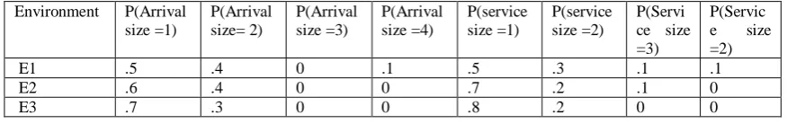
fixed in the three environments E1, E2 and E3 as 𝜆 = 10, 12, 14 𝑎𝑛𝑑 𝜇 = (4, 5, 6). Twelve examples are studied with various values for C, M and N. The maximum arrival size M and the maximum service size N in all environments are (i) M=N=4 in four examples, (ii) M=4, N=3 in four examples studied for Model (A) and (iii) M=3, N=4 in four examples studied for Model (B). In all these sets of different values of M and N, mentioned in (i), (ii) and (iii) the number of servers C are varied as C = 3, 4, 6 and 7. When M=N=4 the probabilities of bulk
arrival and bulk service sizes in the environments are as follows given in Table1.
Table 1: Probabilities of χ Arrival and ψ Service Sizes with Maximums = 4 in Three Environments. Environment P(Arrival
size =1)
P(Arrival size= 2)
P(Arrival size =3)
P(Arrival size =4)
P(service size =1)
P(service size =2)
P(Servi ce size =3)
P(Servic e size =2)
E1 .5 .4 0 .1 .5 .3 .1 .1
E2 .6 .4 0 0 .7 .2 .1 0
E3 .7 .3 0 0 .8 .2 0 0
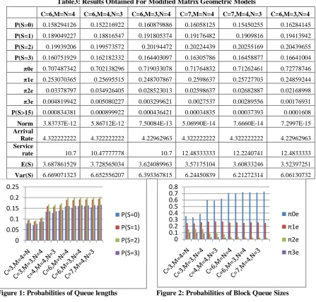
For the cases with M=3, without changing the arrival size probabilities given above in Table 1 for the environments E2 and E3, the arrival size probabilities in E1 are changed as follows P(Arrival size =1 ) =.5 P(Arrival size =2) =.4, P(Arrival size=3)= .1 and P(Arrival size =4) =0. For the cases with N=3, without changing the service size probabilities given above in Table 1 for the environments E2 and E3, the service size probabilities in E1 are changed as follows P(Service size =1 ) =.5 P(Service size =2) =.3, P(Service size =3)= .2 and P(Service size = 4) =0. Here same numbers of 30 iterations are performed to find the rate matrix R in all the twelve cases. When C =3 and C =4 matrix geometric results are seen and the results obtained are presented in Table2. When C= 6 and C=7 modified matrix geometric results are seen and the results obtained are presented in Table 3. Probabilities of various sizes of queue lengths S = 0, 1, 2, 3 and various blocks 0, 1, 2, 3 are obtained. Further P(S> 15), E(S) and VAR (S) are also derived for all the twelve cases. Norms, arrival rate and service rate values are presented. Figure 1 and figure 2 present probabilities of various queue sizes and block sizes for the twelve examples. Effects of variation of rates on expected queue length and on probabilities of queue lengths are exhibited in tables 2 and 3 respectively. The decrease in arrival rates (so also increase in service rates) makes the convergence of R matrix faster which can be seen in the decrease of norm values.
Table2: Results Obtained For Matrix Geometric Models.
C=3,M=4=N C=3,M=4,N=3 C=3,M=3,N=4 C=4=M=N c=4,M=4,N=3 C=4,M=3,N=4 P(S=0) 0.079684166 0.072645296 0.086694481 0.134207116 0.127898311 0.138717179
P(S=1) 0.094816229 0.089299727 0.103026395 0.160159184 0.158139375 0.165224098
P(S=2) 0.099972009 0.094739563 0.10844421 0.168932101 0.167596052 0.173956131
P(S=3) 0.080822795 0.077354801 0.088540336 0.1362632 0.136279652 0.141667691
π0e 0.3552952 0.334039388 0.386705422 0.599561601 0.589913389 0.619565098
π1e 0.246062643 0.239774491 0.258608447 0.269420604 0.27246095 0.268090953
π3e 0.093923215 0.098003396 0.086467581 0.028918419 0.030765921 0.023368742
P(S>15) 0.153006976 0.175220381 0.118796643 0.014310924 0.015827493 0.009800274
Norm 8.607020E-05 0.000121229 5.72322E-05 1.70312E-07 2.66577E-07 6.89660E-08
Arrival
Rate 4.322222222 4.322222222 4.22962963 4.322222222 4.322222222 4.22962963
Service
rate 5.35 5.238888889 5.35 7.133333333 6.985185185 7.133333333
E(S) 8.177499726 8.832269818 7.221716529 3.754933893 3.853312418 3.52779164
Var(S) 69.84639946 81.04471283 53.74109494 13.38646744 13.99187868 11.37540035
Table3: Results Obtained For Modified Matrix Geometric Models
C=6,M=N=4 C=6,M=4,N=3 C=6,M=3,N=4 C=7,M=N=4 C=7,M=4,N=3 C=6,M=3,N=4 P(S=0) 0.158294126 0.152216922 0.160879886 0.16058125 0.15450255 0.16284145
P(S=1) 0.189049227 0.18816547 0.191805374 0.19176482 0.1909816 0.19413942
P(S=2) 0.19939206 0.199573572 0.20194472 0.20224439 0.20255169 0.20439655
P(S=3) 0.160751929 0.162182332 0.164403097 0.16305786 0.16458877 0.16641004
π0e 0.707487342 0.702138296 0.719033078 0.71764832 0.71262461 0.72778746
π1e 0.253070365 0.25695515 0.248707867 0.2598637 0.25727703 0.24859244
π2e 0.03378797 0.034926405 0.028523013 0.02598637 0.02682887 0.02168998
π3e 0.004819942 0.005080227 0.003299621 0.0027537 0.00289556 0.00176931
P(S>15) 0.000834381 0.000899922 0.000436421 0.00034835 0.00037393 0.0001608
Norm 3.83737E-12 5.86712E-12 7.50084E-13 5.06990E-14 7.6660E-14 7.2997E-15
Arrival
Rate 4.322222222 4.322222222 4.22962963 4.322222222 4.322222222 4.22962963
Service
rate 10.7 10.47777778 10.7 12.48333333 12.2240741 12.4833333
E(S) 3.687861529 3.728565034 3.624089963 3.57175104 3.60833246 3.52397251
Var(S) 6.669071323 6.652556207 6.393367815 6.24450839 6.21272314 6.06130732
Figure 1: Probabilities of Queue lengths
Figure 2: Probabilities of Block Queue Sizes
V. CONCLUSION
Two M/M/C bulk arrival and bulk service queues and their sub cases with randomly varying environments have been treated. The environment changes the arrival rates, the service rates, and the probabilities of sizes of bulk arrivals and bulk services. Matrix geometric and modified matrix geometric results have been obtained by suitably partitioning the infinitesimal generator by grouping of customers and environments together respectively when the number of servers is not greater than or greater than the maximum of the maximum arrival and maximum service sizes. The basic system generators of the queues are block circulant matrices which are explicitly presenting the stability condition in standard form. Numerical results for
0 0.05 0.1 0.15 0.2 0.25
P(S=0)
P(S=1)
P(S=2)
P(S=3)
0 0.1 0.2 0.3 0.4 0.5 0.6 0.7 0.8
π0e
π1e
π2e
various bulk queue models are presented and discussed. Effects of variation of rates on expected queue length and on probabilities of queue lengths are exhibited. The decrease in arrival rates (so also increase in service rates) makes the convergence of R matrix faster which can be seen in the decrease of norm values. The variances also decrease. Bulk PH/PH/C queue with randomly varying environments causing changes in sizes of the PH phases may produce further results if studied since PH/PH/C queue is a most general form almost equivalent to G/G/C queue.
VI. ACKNOWLEDGEMENT
The second author thanks ANSYS Inc., USA, for providing facilities. The contents of the article published are the responsibilities of the authors.
VII. REFERENCES
[1] Rama Ganesan, Ramshankar.R and Ramanarayanan. R (2014) M/M/1 Bulk Arrival and Bulk Service Queue with Randomly Varying Environment, IOSR-JM, Vol.10,Issue 6, Ver III, Nov-Dec, 58-66
[2] Ramshankar.R, Rama Ganesan and Ramanarayanan.R (2015) PH/PH/1 Bulk Arrival and Bulk Service Queue ,IJCA, Vol. 109,.3, 27-33..
[3] D. Bini, G. Latouche, and B. Meini. 2005. Numerical methods for structured Markov chains, Oxford Univ. Press, Oxford.
[4] Chakravarthy.S.R and Neuts. M.F.2014. Analysis of a multi-server queueing model with MAP arrivals of customers, SMPT, Vol 43, 79-95,
[5] Gaver, D., Jacobs, P., Latouche, G, 1984. Finite birth-and-death models in randomly changing environments. AAP. 16, 715–731
[6] Latouche.G, and Ramaswami.V, (1998). Introduction to Matrix Analytic Methods in Stochastic Modeling, SIAM. Philadelphia.
[7] Neuts.M.F.1981.Matrix-Geometric Solutions in Stochastic Models: An algorithmic Approach, The Johns Hopkins Press, Baltimore
[8] Neuts. M.F and Nadarajan.R, 1982. A multi-server queue with thresholds for the acceptance of customers into service, Operations Research, Vol.30, No.5, 948-960.
[9] Noam Paz, and Uri Yechali, 2014 An M/M/1 queue in random environment with disaster, Asia- Pacific Journal of OperationalResearch01/2014;31(30.DOI:101142/S02175959 1450016X