A Novel Hyper-parameters Selection Approach for Support Vector Machines to Predict Time Series

A Novel Hyper-parameters Selection Approach

for Support Vector Machines to Predict Time

Series

Yanhua Yu,

The school of Computer Science and Technology, Beijing University of Posts and Telecommunications, Beijing 100876, China

Email:[email protected]

Meina Song and Junde Song

The school of Computer Science and Technology, Beijing University of Posts and Telecommunications, Beijing 100876, China

Email: {mnsong, jdsong}@bupt.edu.cm

Abstract—We propose a novel approach of hyper-parameters selection for SVM regression when it is employed to make time series prediction. In this method, optimal hyper-parameters for SVM are obtained when the residual of training set follows white noise distribution. This conclusion is deduced from the fact that the targets of training set have inherent correlations with each other in time series which is different from other regression problems where the targets of training set are identically and independently distributed. Furthermore, by using this approach, confidence interval can be computed under any given confidence degree 1−α which is an important value for many applications. Two algorithms to compute confidence interval are listed in different cases. At last we compare the prediction results on two benchmark time series with cross validation method.

Index Terms—support vector machines, hyper-parameter, time series prediction, white noise

I.INTRODUCTION

With the development of database and data mining technology, time series prediction have been widely used in financial prediction, electric utility load forecasting, weather and environmental state prediction, communication network traffic prediction. The series of models including ARMA, ARIMA and SARIMA can be used in linear and stationary time series [1]. However, in reality, there are many time series where the underlying system processes are typically nonlinear, non-stationary and not defined a-priori. In this case, SVM and artificial neural network based prediction techniques should be employed [2].

It has been proven that SVM outperform ANN. ANN is based on the principle of Empirical Risk Minimization (ERM), therefore its generalization result can not be guaranteed. Moreover there are some intrinsic troubles such as the long training time, possibility of being stuck into local minima, etc. As for SVM, owing to its solid

theoretical foundation of VC theory and Structural Risk Minimization(SRM)[3]-[4] , it is becoming a more and more promising approach for regression containing time series prediction [5]-[9].

As [5] pointed out, although SVM used for time series prediction span many practical application areas, there appears to be several challenges associated with the use of SVM, among which is the free parameter selection. Hyper-parameters are formulation of SVM contains some such as the kernel parameter, the regularization parameter that control the generalization performance of SVM and

ε

-insensitive zone which determines the number of support vectors. But till now there is no universal method for hyper-parameter selection. If one is using arbitrary SVM parameters, the performance of SVM could be different in a wide range. Finding the optimal hyper-parameters with a good generalization performance is crucial for the successful application of SVM.

There are some investigations on how to set proper values for hyper-parameters [10-17]. The proposed approaches can be summarized as follows:

Smola et al [12] and Kwok [11] proposed asymptotically optimal

ε

−

values

proportional to noise variance.

In [13] parameter C is selected equal to the range of output values. [14] presented improved hyper-parameter selection approach using statistical theory based on [11-13]. [16] used K-fold Cross Validation (KCV) for parameter choice. [17] proposed Leave One Out(LOO).

approach is based on the fact that there are inherent correlations between the targets in training set, which is different from common regression problem where the targets are assumed independent with each other.

This paper is organized as follows. Section 2 gives a brief introduction to SVM regression. In section 3 we describes the proposed approach to selecting SVM regression hyper-parameters. This section also gives two confidence interval calculation methods when SVM model is used to make one-step ahead time series prediction which is an important parameter for many implementations. Section 4 describes experiments applying the proposed approach in two benchmark time series: annual sunspot number and Mackey-Glass. We compare the experimental results with that using simple cross-validation technique. The empirical comparison demonstrates the advantages of the proposed approach. Summary is given in section 5.

II.SUPPORT VECTOR MACHINES

The classical statistics is based on the assumption of infinite samples, but in reality there are only finite samples available. That’s why the overfitting of ANN occurs. V. N. Vapnik and his colleagues proposed Statistical Learning Theory (SLT). STL considers both complexity of estimation function and prediction error on training set with the aim of getting the minimal expectation risk. It is called Structural Risk Minimization (SRM) principle [5]. SVM is just a kind of machine learning method based on this principle. The complete theory foundation wins SVM including SVC (Support Vector Classification) [18] and SVR (Support Vector Regression) widespread attention in application.

The goal of SVR is to estimate an unknown continuous-valued function f( )x based on a finite number set of samples ( , )x_i y_{i with} d

,

i

R y

R

∈

∈

x

_i .

The function f( )x best characterize the regulation underlying the data which makes the equation established:

y=f( )+e (1)

x

.

ε is additive zero mean noise with variance _σ2 _[15].

No matter the target function is a linear or a non-linear function, it can be expressed in the following formulation:

( ) (

( ))

(2)

f

x

=

w

⋅

φ

x

+

b

This equation means even if the estimation function is a non-linear one in input space, it can be viewed as a linear one in feature space F.[6] In equation (1), w∈_{F is the}

coefficient vector, and b R∈ is the bias.

To find the best estimation function, SVM not only pursue the minimization of empirical loss on training set, but also pursue the minimization of the function complexity. Obeying this SRM principle, SVM constructs optimal model by solving the following optimization problem with some inequalities constraints:

( )

(

)

(

)

(

)

(

)

* 2 * , , 2 * 1 * *

min

( , , )

1

1

|| ||

(

)

2

s.t.

( )

; 1,2, ,

( )

; 1,2, ,

0; 1,2, ,

0; 1,2, ,

n l

w R b R R

l

i i

i

i i i

i i i

i i

R

C

l

b

y

i

l

y

b

i

l

i

l

i

l

ξ

ξ ξ

ξ ξ

φ

ε ξ

ε ξ

ξ

ξ

∈ ∈ ∈ =

=

+ ⋅

+

⋅

+ − ≤ +

=

⋅⋅⋅

−

⋅

+ ≤ +

=

⋅⋅⋅

≥

=

⋅⋅⋅

≥

=

⋅⋅⋅

∑

w

w

w

x

w x

(3)

The optimization function in Eq.(3) contains two parts: * 1

1

(

)

l i i i

l

=

ξ ξ

+

∑

is the empirical loss using ε

-insensitiveness loss function; the other part 1 _{|| ||}2

2 w is the margin which represent the bound of VC dimension designating complexity. There are some parameters to be manually set including C,

ε

. These parameters are called hyper-parameter or meta-parameter. The regularization constant C (>0) determines the tradeoff between the empirical error and the complexity term.

ε

is the parameter for the

ε

-insensitive loss function which is a new type of loss function proposed by Vapnik[4][5]:

0 if y-f(x)

( , ( ))

y-f(x)

if y-f(x)

L y f x

_ε

ε

ε

ε

⎧

≤

⎪

=⎨

−

>

⎪⎩

(4)

This loss function is the most commonly used at present. So

ξ

i and

* i

ξ

are called slack variables measuring the deviation of training samples outside

insensitive

ε

− zone.

To solve the optimization problem aforementioned in equation (3), Lagrange dual principle is used. Thus the original problem is transformed to this problem where

( )*

α

are the Lagrange multipliers.

(

)(

)(

)

(

)

(

)

(

)

* * 1 1 * * 1 1 * 1 *

1

min

( ) ( )

2

(5)

. .

0

0

,

l l

i i j j i j i j

l l

i i i i i

i i l i i i i i

y

st

C

l

α α α α φ

φ

ε α α

α α

α α

α α

= = = = =

−

−

⋅

+

+ −

−

−

=

≤

≤

∑∑

∑

∑

∑

x

x

This is a quadratic optimization problem with linear function constraints, and there must be globally minimal value. Many approaches have been proposed to calculate the coefficients _α( )* _{including chunking,}

equation:

(

*

)

1

(

)

l

i i i

i

α

α φ

=

=

∑

−

w

x

. (6)

From this equation we can obtain the conclusion that only those input vectors with

(

*

)

i i

α −α not equal to zero have effects on

w

, and w are completely determined by these input vectors. That is why the learning method is called Support Vector Machines. The parameter b in the decision function can be derived by Karush-Kuhn-Tucker (KKT) condition.

But the mapping function φ

( )

x is not easy to be

found. Furthermore, there is so-called ‘curse of dimensionality’ in the high dimensional feature space F. So the concept of kernel function is proposed which can make Eq.(5) be transformed to the following:

(

)(

) (

)

(

)

(

)

(

)

* * 1 1 * * 1 1 * 1 *

1

min

,

(7)

2

. .

0

0

,

l l

i i j j i j

i j

l l

i i i i i

i i l i i i i i

K

y

s t

C

l

α α α α

ε

α α

α α

α α

α α

= = = = =

−

−

+

+

−

−

−

=

≤

≤

∑∑

∑

∑

∑

x x

And the approximation function for the nonlinearly separable problem is:

(

*

)

(

)

1

( ) l _{i i i}, (8 )

i

f x

α

α

K b

=

=

∑

− x x + Accord

ing to the principle of Hilbert-Schmidt, all the operators satisfying Mercer condition can be used as kernel function. he most commonly used kernel functions include:

Polynomial kernel

' '

( , ) ((

) ) is positive integer (9)

d

K x x

= ⋅ +

x x

c

d

Gaussian Radial Basis kernel 2

' '

( , ) exp(

) (10)

K x x

=

−

γ

x

−

x

Sigmoid kernel '

( , ) tanh( (

i j

)

) (11)

K x x

=

b x x

⋅

+

c

III.PROPOSED APPROACH FOR SVM PARAMETER

SELECTION

There are 3 steps to make time series prediction using SVM. Firstly, phase space should be reconstructed where the embedding dimension is the key value to be determined. Secondly, proper hyper-parameter values should be selected and a best model then can be constructed. At last, prediction steps should be given and prediction values and confidence interval then can be computed.

Next, the above three steps will be discussed in several subsections.

A. Phase Space Reconstruction Of Time Series

Let a time series

x x

₁

, , , ,

₂

_L

x

_i

_L

x

_N denote observations made at equidistant time intervals

0

h

,

0

2 , ,

h

0

ih

, ,

0

Nh

τ

+

τ

+

_L

τ

+

_L

τ

+

, where

x

_i denotes observation at time τ0+ih if we adopt τ0 as the

origin and h as the unit of time. Time series prediction

means to predict a future value

t k

x

₊ at time point

0 (t k h)

τ + + by using the given time series. So the work is to find the relation between

i

x

and values at the time points prior to it including

1 2

{ , ,

x x

_{i− i−}

L

x

_{i m−}

}

. This relation is usually called

model. To get the model according to the given time series, a transformation should be carried to transform the original time series to a series where the items are all points with m-dimension input and 1-dimension output denoted by

( ( ), ( ))

x

i y i

. The parameter m is called embedded dimension. The transformation will be carried as following:

1 2

2 3 1

( 1) 1

...

(1)

...

(2)

...

...

(

)

m m

N m N m N

x

x

x

x

x

x

x

x

x

N m

+ − − − −

⎡

⎤ ⎡

⎤

⎢

⎥ ⎢

⎥

⎢

⎥ ⎢

⎥

=

_⎢

=

⎥ ⎢

⎥

⎢

⎥ ⎢

₋

⎥

⎢

⎥ ⎣

⎦

⎣

⎦

x

x

X

x

L

1 2

(1)

(2)

...

(

)

m m N

x

y

x

y

x

y N

m

+ +

⎡

⎤

⎡

⎤

⎢

⎥

⎢

⎥

⎢

⎥

⎢

⎥

=

=

⎢

⎥

⎢

⎥

⎢

⎥

⎢

₋

⎥

⎣

⎦

⎣

⎦

Y

So our task is to find the function f between input

X

and output

_Y

enabling (

y i

( )

=

f

( ( ))

x

i

) established. In the process, the value of parameter m _{is a key}

problem. There are no uniform algorithm to compute it, and the most commonly used is the method called FPE(Final Prediction Error). In our experiment FPE method is adopted.

B. Prediction Steps Determination

Time series prediction means to predict a future value

t k

x

₊ at time point τ0+ +(t k h) by using the given

time series. The numbers of steps to be predicted is decided by user. When k is equal to 1, it is called

one-step ahead prediction, while ifk>1 it is called

C. Parameters and Model Selection

The advantage of SVM including automatically deciding network structure and finding global optimum are under the premise of given value of free parameters, in other words, if the parameters are different, the network structure and model will be different. From the above eq. (1) it can be seen that these free parameters are

ε

, trade-off parameter C and mapping function φ(x )_.

Because the (φ x ) is difficult to find and therefore it is often replaced by K(xi,xj), what we should do is to find the kernel function K x x( ,i j).

There were some researches on selecting kernel function [19]. The basic conclusion is the Radial Basis Function (RBF) is the first option when there is little prior knowledge since it has good approximation result in both linear and nonlinear system. RBF kernel is the most commonly explointed.

Next work is to select the appropriate

γ

, C and

ε

. There were some papers on this topic [10-17]. But most of them are not fit for time series. The most commonly used for time series modeling are cross-validation and Least Squared Error (LSE) on validation set. But there are problems in using LSE of validation set because this principle is also based on the classical statistical ERM which is substituted by SRM.

Our goal is to find a function _{f x( )} to make the

following equation established:

( )

y = f x + e .Considering the fact that the targets of

training set are in inherent correlations with each other when they are used to model time series, which is totally different from other areas where it is assumed that the target values are independent with each other, an additive constraint should be added to the training of SVM. This constraint is the residual of the training sample should be a white noise. T The condition is that the residual

ε

of the training items should be white noise process. Otherwise it implies that there is still some information left away because of underfitting, or overfiting happened which led to faked correlation.

The method of checking white noise is based on Theorem 1.

Theorem 1. If a time series is a white noise process satisfying the distribution: _{~ (0,} 2₎

t

Z WN σ , The jth lag

autocorrelation coefficient denoted by rjmust follow normal distribution which can be expressed as

1 ~ (0, ) j

r N

n .

To check if a time series is a white noise process, what we should do is to check if no rj satisfies

j

r 2

n

> according to Normal distribution under

confidence degree 1− =α 0.95. If there is a value of j satisfying rj

2

n

> , then it is not white noise and the

model should not be selected. Certainly, the value of lag j

should not be too large, generally the value of j for rj being checked should be less than

3

n or n.

Here we use a branch of SVM called ν−SVM[10].

Instead of setting the value of

ε

, we set the value of

ν _{( 0≤ ≤ν 1) which can then acquire the value of}

ε

_{automatically.}

Figure 1. Hyper-parameter selection for SVM using proposed white noise constraint

D. Confidence Interval Calculation

As white noise process is commonly regarded as following normal distribution, the confidence interval can be calculated under a given confidence degree. Taking confidence degree as 1− =α 0.95, we can get the confidence interval of ( 2 )± σ and confidence bound

of ( ^ ^

( (y n+1) 2 , (− σ y n+1)+2 )σ ). If confidence degree is taken as 1− =α 0.97,the confidence interval will be ( 3 )± σ and confidence bound will be

^ ^

( (y n+1) 3 , (− σ y n+1)+3 )σ where

σ

is the standard deviation of residual. If the numbers of training items is larger than 50 the standard deviation

2

1 1

( )

1 k

i i

S e e

k =

= −

−

∑

of sample can be

considered as equal to the global standard deviation

σ

. But if the number of data points in training sample is smaller, the value of

σ

and S may vary much. In this condition, the following algorithm should be taken.

Let a residual sequence be denoted by

{ }

e

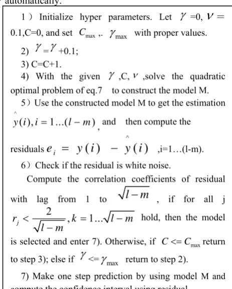
_i which satisfy normal distribution, and its mean value denoted

1）Initialize hyper parameters. Let

γ

=0,

ν

＝

0.1,C=0, and set Cmax,.

γ

max with proper values.

2)

γ

=

γ

+0.1; 3) C=C+1.

4) With the given

γ

,C,ν ,solve the quadratic optimal problem of eq.7 to construct the model M.

5）Use the constructed model M to get the estimation ^

( ), 1...( )

y i i= l−m _{, and then compute the}

residuals

^

( )

( )

i

e

=

y i

−

y i

,i=1…(l-m). 6）Check if the residual is white noise.

Compute the correlation coefficients of residual with lag from 1 to

l

−

m

, if for all j

2

, 1... j

r k l m

l m

< = −

− hold, then the model

is selected and enter 7). Otherwise, if C<=C_maxreturn to step 3); else if

γ

<=

γ

_max return to step 2).

by

_e

−also satisfies normal distribution:

2

~ (0,

)

e

N

n

σ

−

.

According to the linear operational characteristics of normal distribution variables, The stochastic variable

1 n

e

e

−

+

−

will also satisfy normal distribution: 2

1 2

1

~ (0,[1

] )

n

e

e

N

n

σ

−

+

−

+

(12)

and this is equivalent to equa.(13):

1 2

2

~ (0,1) (13) 1 n e e W N n n σ − + − = + It is well known that the sample variance 2

S

follows X2 distribution: 2 2 2

(

1)

~

(

1) (14)

n

S

Z

X

n

σ

−

=

−

,

Combine the aforementioned equation (13) and equation (14), a variable named Z satisfying Student’s

distribution can be obtained:

~ (

1)

(

1)

W

t n

Z n

−

−

(15)

Substitute the equation (15) in (13) and (14), we acquire the following equation:

1 2 2 2 1 2 1

. ~ ( 1) (16) 1 n n e e n e e n n t n

S n S

σ σ − + − + − + − = − +

Let confidence degree is 1−α , We can get the following formulation:

2 1 2

2 2

{ ( 1)

.

( 1) }=1- (17)

1

n

e

e

n

P t n

t n

n

S

α α

α

− +

−

− − ≤

≤

−

+

It can be transformed to equation (18):

2 2 1 2 2 2 2

1

1

{

n

( 1)

_n

n

( 1) }=1- (18)

Pe

t n S e

e

t n S

n

α

n

α

α

− −

+

+

+

−

− ≤ ≤ +

−

Integrate equation (18) and equation (1), we can get the following equation:

2 ^ 2 2 2 _^ 2 2 1

{ ( 1) ( 1) ( 1)

1

( 1) ( 1) }=1-

n

P e t n S y n y n n

n

e t n S y n n α α

α

− − + − − + + ≤ + + ≤ + − + + (19) .

IV.EXPERIMENTS AND RESULTS ANALYSIS

A. Annual Sunspot Number

Annual sunspot number data is generally regarded as classical nonlinear non-stationary time series which is often used to compare and assess statistical model and prediction method [20]. To make results comparable, this study uses the same experimental setup as used in [21][22][23].The only difference is that in our experiment, the annual sunspot number from 1700 to 1955 is taken as training data, and the data points from 1956 to 1979 are used as test data. Softwares employed are Matlab7.1 and Libsvm2.83 [24] which is embedded to the prior to carry out iteration control.

(1) To reconstruct phase space from original time series. The critical problem is to determin embedded dimension

m

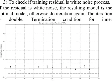
. Using C-C approach, the embedded dimension is calculated as 5.

(2) To construct the optimal model on the training sample by using SVM. The sign of the best model is that the training residual satisfying white noise form. The details are as follows.

1）

γ

＝0.1, C=1.

2) To construct a model with the current values of hyper-parameter

γ

and c.

3) To check if training residual is white noise process. If the residual is white noise, the resulting model is the optimal model, otherwise do iteration again. The iteration is double. Termination condition for inner

Figure 2. Autocorrelation function of training residual

iteration is C=2000, and the step size for C is 1. Termination condition for outer iteration is

γ

=10. The first pair of

γ

and C is (

γ

=0.4, C=1313) and the autocorrelation function is depicted in Fig. 2

(3)To make prediction and evaluate the results.

The one-step predicted value for year 1956 is

1956

109.9

x

=

^

. The actual value for year 1956 is

1 9 8 0 1 4 1 .7

x = . Fig.3 shows the predicted and actual

sunspot numbers from 1956 to 1979. From this figure it can be seen that the predicted and actual values are similar and have the same trend. A more detailed results and analysis is shown in TABLE I. In this table, NMSE is the most commonly used to evaluate annual sunspot series prediction and its meaning is list as follows.

2 1

^

1 ₂

( l

₍

₎

)

i

NMSE

l

y

_i

y

_i

δ

=

2

1 1

2

( )

1

(

)

l

i

l

y

_i

y

δ

=

− =

−

∑

−

TABLEI

ANNUALSUNSPOTNUMBERPREDICTIONFOR1956TO1979

Methods NMSE SVM with White Noise constrained 15%

Benchmark[21] 15.4% Benchmark[22] 35% Benchmark[23] 28%

Figure 3. The predicted and actual values of annual sunspot numbers in 1956~1979

TABLE I shows that the value of NMSE by using white noise constrained SVM is 0.15 which is a better or comparable prediction than results shown in [21]-[23]. What’s more, since the residual is white noise process which is commonly regarded as following normal distribution, we can get confidence interval under any confidence degree 1−α by using Normal distribution or Student’s distribution. This feature is specifically important to those applications where a confidence bound is needed other than a single prediction value.

B. Mackey-Glass

Our second application is a high dimensional chaotic system generated by the Mackey Glass delay differential equation

10

0.2 (

)

( )

0.1 ( )

(20)

1

(

)

d d

x t

t

dx t

x t

dt

x t

t

−

= −

+

+

−

With delay

t

_d

≥

17

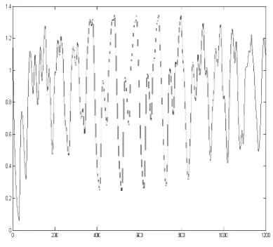
. Eq. (20) was originally introduced as a model of blood cell regulation and became quite common as artificial forecasting benchmark[7][17].

Figure 4. 1200 points of the Mackey-Glass time series MG17

We obtained training set (600 patterns) using an embedding dimension m=6 and step size κ =6. So

( )t

Χ is used to predict x t( +κ), and the whole dataset can be split into 6 independent datasets: the first one S1

containing

x

_{1 ( 1)+ −d κ} , the second one S2 containing 2 (d 1 )

x _{+ − κ , L , and the last, that is, the sixth} 6

S

containing

x

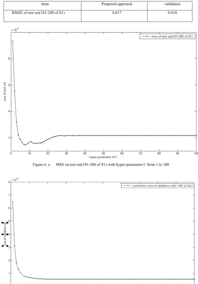
_dκ. A common training method is as shown in [17]: The first 100 points of S1 are used as

hyper-parameters. In this paper, we use the proposed approach to model the same dataset. Every dataset is used as the training set, and hyper-parameter is also selected using the set itself. Using the procedure shown in Fig. 1, we trained the dataset S1 and get the pair of

γ

and C with

γ

=0.7

, C=7. The prediction value is 0.9699 and the actual value is 0.9639. Repeat the method above, we can get the prediction values for the succeeding 12 data points. The prediction results are shown in TABLE II. To compare the proposed approach with the method of LSE, we also make prediction using the latter. The prediction results for the same dataset are shown in TABLE III. This table shows that the performance of the proposed approach is better than the classic one: about 0.002 smaller. Fig. 6.a and 6.b depict the cause of this difference. From Fig. 6.a, we can see

that the minimal of MSE for test set appears when C is between 8 and about 17. But fig. 6.a shows that as C becomes greater, the MSE for validation set steadily become smaller until it converges into a fixed value. By using the validation set LSE method, we will select a value of C larger than 20,for example we can select C=40. But using the approach proposed in this paper, since white noise of training residual appears when C=7 and C=8, From these two figures we can get the prediction MSE on test set shown in TABLE III. And similar results can be abtained by using other sets. The statistic MAPE

means

1

^ 1

( n

|

|

)

i

i i

M A P E n

i

y

y

y

=

=

∑

−

TABLEII

ANALYSISOFANNUALSUNSPOTNUMBERPREDICTIONRESULT

Item 101 102 103 104 105 106 107 108 109 110 111 112

Actual value

0.9 643

0.9 749

0.9 78

0.9 749

0.9 668

0.9 545

0.9 391

0.9 21

0.9 009

0.8 792

0.8 56

0.8 318 Predicti

on value(1S)

0.9 688

0.9 902

0.9 825

0.9 692

0.9 575

0.9 434

0.9 392

0.9 218

0.8 951

0.8 75

0.8 525

0.8 269 Confide

nce interval(97 %)(

±

)

0.0 078

0.0 371

0.0 290

0.0 253

0.0 211

0.0 305

0.0 057

0.0 072

0.0 288

0.0 237

0.0 213

0.0 214

Absolut e error

0.0 045

0.0 153

0.0 045

-0. 0057

-0. 0093

-0. 0111

0.0 001

0.0 008

-0. 0058

-0. 0042

-0. 0035

-0. 0049 Relevan

t error(%)

0.4 6

1.5 6

0.4 6

-0. 58

-0. 96

-1. 16

0.0 1

0.0 8

-0. 64

-0. 47

-0. 40

-0. 58 RMSE 0.0071 MAPE(

%)

0.0058 Note: 1S means one step ahead prediction

TABELIII

COMPARISONOFMSEONTESTSET(101-200POINTSOFS1)BETWEENCROSSVALIDATIONANDTHE NEWAPPROACH

Item Proposed approach validation

RMSE of test set(101-200 of S1) 0.017 0.018

Figure 6. a MSE on test set(101-200 of S1) with hyper-parameter C from 1 to 100

V.CONCLUSION

Time series prediction is widely used in many areas. In this paper, the problem of selecting optimal hyper-parameters is deeply explored when SVM is used in time series prediction. A novel approach is proposed which is aimed to make the training residual white noise regarding that the target values in training set have inherent correlations with each other. Exploiting this novel method we can compute the confidence interval under any given confidence degree 1−α which is very important to many applications. Experiments have been taken on two typical nonlinear non-stationary time series-annual sunspot number series and Mackey-Glass. The experiments demonstrate the advantage of the proposed approach. Certainly this approach can also be applied for linear or stationary time series prediction, but it is not proper for domains other than time series.

ACKNOWLEDGEMENT

This work is supported by the National Key project of Scientific and Technical Supporting Programs of China (Grant No. 2009BAH39B03); the National Natural Science Foundation of China (Grant No.61072060); the National High Technology Research and Development Program of China (Grant No. 2011AA100706); the Program for New Century Excellent Talents in University (No.NECET-08-0738); the Research Fund for the Doctoral Program of Higher Education(Grant No. 20110005120007); the Co-construction Program with Beijing Municipal Commission of Education; Engineering Research Center of Information Networks, Ministry of Education.

REFERENCES

[1] George E.P. Box, Gwilym M Jenkins, Gregory C. Reinsel, Time Series Analysis: Forecasting and control. Beijing: Posts & Telecom Press 2005.

[2] M. Versace, “Predicting the exchange traded fund DIA with a combination of genetic algorithms and neural networks,“ Expert Systems with Applications, 2004, 27(3), pp. 417 – 425.

[3] V. Vapnik, The Nature of Statistical Learning Theory (2nd ed.). Springer, 1999.

[4] V. Vapnik, Statistical Learning Theory. New York: Wiley, 1998.

[5] Nicholas I. Sapankevych, Ravi Sankar., “Time series prediction using support vector machines-a survey,” IEEE Computational Intelligence Magazine, 2009, 5: 28-38. [6] A. Smola and B. Schölkopf, A Tutorial on Support Vector

Regression. Neuro COLT Technical Report NC-TR-98-030, Royal Holloway College, University of London, UK, 1998

[7] K.R. Muller, and A. Smola, “Prediction time series with support vector machines,” Proceedings of International Conference on Artificial Neural Networks, Lausanne, Switzerland, 999, 1997.

[8] U. Thissen, R van Brakel, A P de Weijer, “Using support vector machines for time series prediction,” Chemometrics and Intelligent Laboratory Systems (S0899-7667), 2003, 69, pp. 35-49.

[9] Zhiwei Shi, Min Han, “Support Vector Echo-State Machine for Chaotic time-series prediction,” IEEE Tran. on Neural Networks, 2007, 18(2), pp. 359-372.

[10]B. Schölkopf, P. Bartlett, A. Smola, and R. Williamson, “Support Vector regression with automatic accuracy control,” in L. Niklasson, M. Bodén, and T. Ziemke, ed., Proceedings of ICANN'98, Perspectives in Neural Computing, Springer, Berlin, 1998: 111-116.

[11] J.T. Kwok, “Linear Dependency between

ε

and the Input Noise in

ε

–Support Vector Regression,” in: G. Dorffner, H. Bishof, and K. Hornik (Eds): ICANN 2001, LNCS 2130 (2001) pp. 405-410.

[12]A. Smola, N. Murata, B. Schölkopf and K. Muller, “Asymptotically optimal choice of

ε

–loss for support vector machines,” Proc. ICANN, 1998.

[13]D. Mattera and S. Haykin, “Support Vector Machines for dynamic reconstruction of a chaotic system,” in: B. Schölkopf, J. Burges, A. Smola, ed., Advances in Kernel Methods: SupportVector Machine, MIT Press, 1999. [14]V. Cherkassky, Y. Q. Ma, “Practical Selection of SVM

Parameters and Noise Estimation for SVM Regression “,

Neural Networks, 2004, pp.113-134.

[15]B. Scholkopf, J. Burges, A. Smola, Advances in Kernel Methods: Support Vector Machine. MIT Press, 1999. [16]O. Bousquet, A. Elisseeff, “Stability and generalization,”

Journal of MachineLearning Research, 2002, 2, pp. 499–

526.

[17]Liva Ralavola, Florence d’Alche-Buc, “Dynamical Modeling with Kernels for Nonlinear Time Series Prediction,” Proc. NIPS 13(2001), pp. 981-987.

[18]P. G. V. Axelberg, I. Y. H. Gu, M. H. J. Bollen, “Support Vector Machine for classification of voltage disturbances,” IEEE Tran. On Power Dilivery, 2007, 22(3), pp. 1297-1303.

[19]Haina Rong, Gexiang Zhang, Weidong Jin, “Selection of kernel functions and parameters for support vector machines in system identification,” Journal of System Simulation, 2006, 18(11), pp. 3204-3226

[20]Time Series Prediction group [EB/OL]. http:// www.cis.hut.fi/projects/tsp/?page=Timeseries,2006-05-08. [21]L Cao, “Support vector machines experts for time series

forecasting,” Neurocomputing, 2003, 51, pp. 321- 339. [22]A.S. Weigend, B.A. Huberman, D.E. Rumelhart,

“Predicting the future: a connectionist approach,” Int. J. Neural Systems 1 (1990), pp. 193–209.

[23]H. Tong, K.S. Lim, “Threshold autoregressive, limit cycles and cyclical data,” J. Roy. Statist. Soc. B 42(3) (1980), pp. 245–292.

[24]C. C. Chang, C. J. Lin. IBSVM: a library for support vector machine [J / OL]. Taiwan : [ s. n. ] , 2006[2007-3-20]. http: ∥ www.csie.ntu.edu.tw/ ～

cjlin/libsvm

Dr Yanhua Yu was born in Hebei, China, in 1974. She obtained her Bachelor’s degree, Master’s degree and Doctor’s degree in computer science and technology respectively in 1995, 1998 and 2008 from Beijing University of Posts and Telecommunications, Beijing, China.

evaluation method based on support vector machines”(Journal of Beijing University of Posts and Telecommunications Publishing Press, Beijing, China, 2007), “A mechanism of telecommunication network performance monitoring based on anomaly detection” (Journal of Electronics & Information Technology, 2009), and the first author of “A dynam ic compuation approach to determ ining the threshold in network anomaly detection”(Journal of Beijing University of Posts and Telecommunications, 2011). Her areas of interest include network management and optimization, artificial intelligence and data mining.

Dr Yu received Award for Research Achievements of High Schools by Ministry of Education of the People’s Republic of China, 2010.

Professor Junde Song was born in 1938. He is the Honor Ph.D. of Moscow University, Russia.

He published lots of articles and books in the area of computer and communication network. The most recently published include “A novel bargaining based relay selection and power allocation scheme for distributed

cooperative communication

networks”(Vehicular Techology Conference-VTC,pp.1-5,2010),”Distributed Optimal Relay

Selection for QoS Provisioning in Wireless Multi-Hop Cooperative Networks”, (Global Telecommunications Conference-GLOBECOM,pp.1-6,2009s) and “Utility-based resource allocation and scheduling for CR-MIMO-OFDMA/TDM system”(Journal on Communications, 2010, 31(7), pp. 1-8). His areas of interest include mobile network and its management, artificial intelligence and data mining, modern service science and engineering.