Modified Shuffled Frog-leaping Algorithm with
Dimension by Dimension Improvement
Juan Lin
College of Computer and Information Science, Fujian Agriculture and Forestry University, Fuzhou, China Email: [email protected]
Yiwen Zhong
College of Computer and Information Science, Fujian Agriculture and Forestry University, Fuzhou, China Email: [email protected]
Abstract—Shuffled leap frog algorithm (SFLA) is a new nature-inspired intelligent algorithm, which uses the whole update and evaluation strategy on solutions. For solving multi-dimension function optimization problems, this strategy will deteriorate the convergence speed and the quality of solution of algorithm due to interference phenomena among dimensions. To overcome this shortage, a dimension by dimension improvement based on SFLA is proposed. The proposed strategy combines an updated value of one dimension with values of other dimensions into a new solution, and that whose updated value can improve the solution will be accepted greedily. Further, a new individual update formula is designed to learn experiences both from the global best and the local best solution simultaneously. Meanwhile, they also reveal the modified algorithm is competitive for continuous function optimization problems compared with other improved algorithms.
Index Terms—shuffled leap frog algorithm, dimension by dimension, multi-dimensional function optimization
I. INTRODUCTION
Shuffled frog-leaping algorithm (SFLA) is a stochastic population based optimization algorithm, first published by Eusuff and Lansey in 2003[1]. In SFLA, frogs are seen as hosts for memes and described as a memetic vectors. Each meme consists of a number of memotypes. The monotype represents an idea in a manner similar to a gene representing a trait of a chromosome in genetic algorithm (GA). Based on this abstract model, SFLA draws on a local search, the idea of competitiveness and mixing information from parallel local searches to move toward the global best solution.
Since its first publication, a large body of research has been done to study of the applications of SFLA,
involving the industrial system optimization and control, data mining, radio technology, bioinformatics and soft computing[2-7] etc.
To improve the performance of SFLA, many studies concentrated on a better understanding of the local update formula, the control parameters and the grouping strategy. Ref.[2] introduced a new search-acceleration parameter into the update formula. Bhaduri[8] used a modified
clonal selection and mutation for the best frogs in each population. Zhen et al. [9] proposed a new grouping strategy and made all the frogs participate in the evolvement by keeping the inertia learning behaviors and learning from better ones selected randomly. Li et al.[10] improved the leaping rule by extending the leaping step size and adding a leaping inertia component to account for social behavior. They also introduced the extremal optimization into SFLA to enhance the local search ability. Luo and Chen[11] studied the trajectory and convergence of SFLA, deduced a conclusion that SFLA is global convergent. Their also presented a mutation selection of EO-SFLA to expand the search space. Zhao[12] added an mutation idea in Differential Evolution(DE) algorithm to disturb updating strategy locally. In order to accelerate the convergence, Ding et al. [13] proposed a quantum frog-leaping co-evolution and designed a dynamic multi-cluster frog structure. In view of overcoming the slow searching speed in the late evolution and local minimum, the ideas of simulated annealing(SA) and immune vaccination were involved by Zhang et al. [14]with Gaussian mutation and chaotic disturbance.
From the above studies it can be concluded that the local search strategy is very important in SFLA, the appropriate strategy may improve its performance remarkably. Therefore, a more sophisticated neighborhood search space is necessary. In order to improve the ability of intensification, this paper presents new algorithm with a dimension by dimension improvement. In the progress of local search, the worst frogs in the submemeplexes are updated and evaluated dimension by dimension, and then accepted greedily. The individual update equation is redesigned to absorb good information from the optimal individual within the submemeplex and the global best one concurrently, which contributes to the acceleration of convergence.
approach and results, which were carried on typical benchmark function optimization problems. Finally, section 5 summaries the study.
II.SHUFFLED FROG-LEAPING ALGORITHM
SFLA involves a population of possible solutions arranged according to the fitness, which is divided into several memeplexes. Each memeplex symbolizes a collection of frogs with different memes (ideas), performs simultaneously an independent local search, and moves towards the best solution in the memeplex and the population one. All memeplexes are periodically shuffled and reorganized to exchange the evolutionary information. Local exploration and global shuffling alternate until a pre-defined convergence criterion is satisfied.
Suppose the search space is D-dimensional, then the i-th frog of i-the swarm can be represented by a D -dimensional vector, Xi=(xi1,xi2,…xiD). The frogs are sorted
in a descending order according to their fitness. The whole population is divided into m memeplexes, each comprising n frogs. (i.e. P=m*n, P is the size of the population). Each memeplex is constructed according to the following equations:
{ | ( 1), 1,2,... } 1,2,...
k k k
Y = Xi Xi =Xk m i+ − i= n k= m (1)
where Ykmeans the k-th memeplexes.
To avoid the local optimum, a subset of the memeplex called a submemeplex is considered. The submemeplex selection strategy facilitates the frogs that have higher performance values into the submemeplex with higher weight. The weights are assigned with a triangular probability distribution according to (2):
2( 1 )
( 1)
j
n j
p
n n + − =
+ (2)
where pjis the j-th frog in the memeplex.
Within each memeplex, the frog with the worst fitness in the submemeplex is identified as Xw, the best one as Xb.
Then the step S and new position of Xw are manipulated
according to the following two equations:
S =rand() *(Xb−Xw) (3)
Xw' =Xw S+ −Smax≤ ≤S Smax (4)
where rand() is a uniform random number between 0 and 1; Xw’ is the new position. Smax is the maximum allowed
change in a frogs’ position. If this process produces a better solution, Xw is replaced by Xw’. Otherwise the
calculation is repeated with respect to the global best frog Xg. If there is still no improvement, a feasible solution to
replace Xw is randomly generated. After a specific
number of memetic evolution time loops, the memeplexes are shuffled to enhance the exchange of global information. The main parameters of the SFLA are: number of frogs P, number of memeplexes m, number of iterations within each memeplex N and the maximum leaping size Smax.
III.SFLA WITH ADAPTIVE LEAP DIMENSION
The local exploitation makes the worst frog substantially influenced by the local or global best position, with the maximum step size controlling the fine degree of search. The fitness will be recalculated only when all dimensions of the worst frog have been updated. In this way, the entire individual (all dimensions) is an independent evaluation unit, completely ignores the excellent partial dimensions in the update process, scilicet, the part of dimensions of an individual which may be closer to the global optimum. If the overall fitness was worse than the original one, this part of the information would be discarded, and the frog would move to the next round of modification until re-randomized generation. On the other hand, even the new fitness is better than the old one, some dimensions may be degraded. It is accepted just for the improvement of the overall fitness.
During the memetic evolution within each memeplex, Xw first learns the idea from the best frog within the
memeplex. If the evolution produces a benefit, Xw is
replaced with a new individual. Otherwise the process is repeated with the global best frog. If it still does not produce a better result, Xw is replaced with a random
individual Xr. In this manner, the effective information
from Xb and Xg cannot be learned simultaneously. Further,
if Xw has not been successfully updated by Xb and Xg,
which means the number of function evaluations times (FEs) is wasted. If we update Xw with Xb and Xg at one
step like the speed update equation in PSO (Clerc, 1999), we may make full use of the good information both from Xb and Xg, and save the function evaluation times.
Inspired by the idea of PSO algorithm, we design the step size S generation equation in our compositive learning strategy as follows:
1 1 2 2
( ( b w) ( g w))
S =k c r X −X +c r X − X (5)
2
1 2
2 2 4 , , 4
k= − −φ φ − φ where φ= +c c φ> (6)
where c1, c2 are two positive constants, called cognitive
and social parameter respectively in PSO.
Here we use their control the submemeplex and the global factor. The constriction factor k is a function of c1
and c1 as reflected in (6). r1, r1 are random numbers,
uniformly distributed in [0, 1]. In this way, Xw can be
updated through tracking Xb and Xg simultaneously.
Randomly generator is retained where there is no improvement during above procedure.
Algorithm 1 is the framework of improvement SFLA algorithm updated with dimension by dimension denoted as SFLA-D. Xwnew is used to store the updated position
within each iteration. Xw j-D andX wnew j-D is the original
Figure 1. The Framework of SFLA-D
IV. SIMULATION
There different experiments to access the performance of SFLA-D using the test suite described in Table 1. The test suite consists of 10 unconstrained single-objective benchmark functions with different characteristics. According to their properties, these functions are divided into three groups: unimodal problems, unrotated multimodal problems, rotated multimodal problems[15]. Although the Rosenbrock’s function is listed in the first group, it also can be treated as a multimodel function at high-dimensional problems[16].
The function error value is used to evaluate the performance of the algorithms. With a solution X, the function error value is defined as:
Error Value= f X( )− f X( *) (7)
where X* is the global optimum of the function.
We follow the parameter settings investigated by ELBELTAGI et al.[17]. Population size P=200, the number of memeplexes m =20, the number of local iterations N = 10. The frogs in each submemeplex are 8. Smax is set to 0.4. The maximum number of fitness
evaluations that allowed for each algorithm to minimize the error set 10000*D, where D is the dimension of the problem. Each function is processed for 30 times
The focus of the study is to compare the performance of the proposed SFLA-D with the original SFLA in different experiments. The performance of SFLA-D comparing with other modified SFLAs also present.
A. Performance Evaluation
We compared the SFLA-D and SFLA at dimension D=30 and the results are presented in Table 2 and Table 3 with two performance evaluation criteria. Table 2 were the results of the minimum function error value can be found, recorded in each run and the average and standard deviation(SD) of the error values were calculated. Table 3 were the results of the number of function evaluations (FEs) required to reach an error value less than the accuracy level ε listed in table 1. The average and SD of the number of evaluations were calculated.
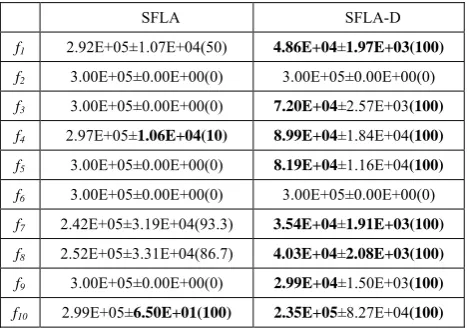
From table 2 we can see, for all kinds of test function, SFLA-D is better than SFLA both with the average and SD of the error values. In addition to f2 and f6, SFLA-D is far superior to SFLA on all functions. Especially on f4 and f5, SFLA-D can always find the global optimal solution within the fixed FEs in 30 runs. And for all functions expect for f2 and f6, SFLA-D reached the target accuracy level successfully using fewer fitness evaluation.
TABLE 1
PERFORMANCES OF COMPARE OF SFLA AND SFLA-D FOR MEAN
ERROR VALUES ACHIEVED (D=30)
SFLA SFLA-D
f1 3.36E-06±3.76E-06 2.54E-57±1.05E-56
f2 1.69E+02±9.85E+01 2.95E+01±1.79E+01
f3 3.55E-02±1.70E-01 2.33E-14±2.75E-15
f4 3.90E-02±3.75E-02 0.00E+00±0.00E+00
f5 1.20E+01±4.71E+00 0.00E+00±0.00E+00
f6 6.33E+03±5.34E+02 1.18E+01±3.61E+01
f7 3.46E-03±1.89E-02 1.57E-32±8.35E-48
f8 1.47E-03±3.80E-03 1.35E-32±5.57E-48
f9 3.82E+03±6.56E+02 5.87E-14±1.82E-14
f10 1.27E+02±1.65E+01 7.05E+00±8.42E+00
TABLE 2
PERFORMANCES OF COMPARE OF SFLA AND SFLA-D FOR MEAN NUMBER OF FES TO ACHIEVE THE ERROR VALUES (D=30)
SFLA SFLA-D
f1 2.92E+05±1.07E+04(50) 4.86E+04±1.97E+03(100)
f2 3.00E+05±0.00E+00(0) 3.00E+05±0.00E+00(0)
f3 3.00E+05±0.00E+00(0) 7.20E+04±2.57E+03(100)
f4 2.97E+05±1.06E+04(10) 8.99E+04±1.84E+04(100)
f5 3.00E+05±0.00E+00(0) 8.19E+04±1.16E+04(100)
f6 3.00E+05±0.00E+00(0) 3.00E+05±0.00E+00(0)
f7 2.42E+05±3.19E+04(93.3) 3.54E+04±1.91E+03(100)
f8 2.52E+05±3.31E+04(86.7) 4.03E+04±2.08E+03(100)
f9 3.00E+05±0.00E+00(0) 2.99E+04±1.50E+03(100)
f10 2.99E+05±6.50E+01(100) 2.35E+05±8.27E+04(100)
Initialize parameter P, m, n, Smax
While (End condition is not met) Sort P in descending order Partition P into m memeplexes For each memeplex T
Repeat the following operation N times Select the submemeplex, Xw and Xb
For each dimension
Calculate position Xwnew using (4)
If f(Xwnew)<f(Xw)
xw j-D=xwnew j-D
End IF
End For
If (No Improved)
Generate a new Xw randomly
Sort T in descending order End Repeat
End For Update Xg
B. Scalability Study
In order to study the effect of dimension on the performance of SFLA-D, a scalability study compared with the original SFLA was presented. Since f9 and f10 are defined up to D=50 dimension, we studied them at D=50 dimension. Other functions were studied at D=50,100 and 200 dimension. We set the same parameters mentioned above. From table 3 we can see SFLA-D is still maintain a good performance, not declined with the increasing dimension. Especially for f5, it still converges to the global optimal solution even on D=200. f4 can converge to the global optimal on D=50 and D=100. Other functions can also converge to an ideal solution.
TABLE 3
PERFORMANCES OF COMPARE OF SFLA AND SFLA-D WITH DIFFERENT
DIMENSIONS
SFLA SFLA-D
D=50
f1 4.21E-06±5.49E-06 2.28E-55±1.23E-54
f2 3.04E+02±2.59E+02 5.61E+01±2.27E+01
f3 5.21E-01±5.88E-01 4.83E-14±3.33E-15
f4 2.79E-02±2.60E-02 0.00E+00±0.00E+00
f5 1.84E+01±5.57E+00 0.00E+00±0.00E+00
f6 1.15E+04±6.98E+02 3.55E+01±5.52E+01
f7 2.78E-05±1.46E-04 9.42E-33±2.78E-48
f8 2.05E-03±4.23E-03 1.35E-32±5.57E-48
f9 3.05E+03±3.88E+02 4.07E-09±1.58E-08
f10 1.57E+02±1.63E+01 5.51E+00±9.52E+00
D=100
f1 7.26E-06±7.18E-06 7.42E-59±2.22E-58
f2 4.46E+02±1.49E+02 9.66E+01±1.37E+01
f3 2.02E+00±3.63E-01 9.49E-14±8.22E-15
f4 2.55E-02±3.23E-02 0.00E+00±0.00E+00
f5 2.98E+01±8.67E+00 0.00E+00±0.00E+00
f6 2.46E+04±9.06E+02 1.58E+01±5.14E+01
f7 3.13E-03±9.83E-03 4.71E-33±1.39E-48
f8 4.41E-03±5.68E-03 1.35E-32±5.57E-48
D=200
f1 4.46E-06±2.42E-06 1.56E-58±4.10E-58
f2 9.13E+02±1.62E+02 1.95E+02±1.49E+01
f3 2.98E+00±2.52E-01 2.08E-13±3.30E-14
f4 4.45E-03±6.23E-03 1.11E-16±0.00E+00
f5 4.24E+01±1.40E+01 0.00E+00±0.00E+00
f6 5.44E+04±2.16E+03 2.55E-03±0.00E+00
f7 1.11E-05±5.93E-06 2.36E-33±0.00E+00
f8 4.97E+00±4.50E+00 1.35E-32±2.88E-48
C. Comparison with Other SFLAs
Table 4 shows the comparison with three other improved SFLA introduced in section I. The first algorithm [2] adds an accelerated factor denoted as MSFLA. The second one [9] proposed a new group and update strategy, we denote as ISFLA. The three one [12]
gets into DE disturbance denoted as SFLADE. The same parameters set to all algorithms expect for the specific parameters in separate.
From table 4 we can see SFLA-D reached smaller error values on f6 and f10, reached the global minimum on f4 and f5 with ISFLA, reached the same error values on f7 and f8 with MSFLA. On f1, SFLA-I reached the global minimum, SFLA-M was better than SFLA-D too. In f2, SFLA-M is best in terms of error value, SFLAI is the best in SD. In f3, SFLAI is the best. And In f9, SFLA-D is only worse than MSFLA with SD. Overall, SFLA-D get the better performance on most of the unrotated multimodal functions and rotated multimodal functions.
TABLE 4
PERFORMANCES COMPARISON WITH OTHER IMPROVED SFLAS
SFLA-D MSFLA
f1 2.54E-57±1.05E-56 1.07E-143±2.78E-143
f2 2.95E+01±1.79E+01 1.52E+01±1.55E+01
f3 2.33E-14±2.75E-15 7.55E-15±1.62E-15
f4 0.00E+00±0.00E+00 3.94E-03±6.95E-03
f5 0.00E+00±0.00E+00 2.02E+01±4.37E+00
f6 1.18E+01±3.61E+01 5.26E+03±7.20E+02
f7 1.57E-32±8.35E-48 1.57E-32±8.35E-48
f8 1.35E-32±5.57E-48 1.35E-32±5.57E-48
f9 5.87E-14±1.82E-14 5.12E-14±1.73E-14
f10 7.05E+00±8.42E+00 1.02E+02±1.71E+01
ISFLA SFLADE
f1 0.00E+00±0.00E+00 2.42E-04±9.17E-05
f2 2.89E+01±1.91E-02 6.01E+01±6.42E+01
f3 4.44E-16±0.00E+00 1.15E+00±8.44E-01
f4 0.00E+00±0.00E+00 1.23E-02±9.68E-03
f5 0.00E+00±0.00E+00 1.53E+01±4.67E+00
f6 8.49E+03±1.82E+02 4.08E+03±1.33E+03
f7 7.86E-01±1.58E-01 6.95E-03±2.63E-02
f8 2.88E+00±3.17E-02 6.95E-03±7.14E-03
f9 5.97E+04±4.14E+03 7.39E-01±3.52E-01
f10 3.75E+02±1.83E+01 7.87E+01±2.54E+01
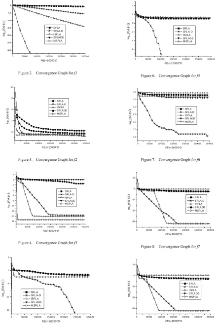
D. Iteration Process for Fixed FEs
Figure 2. Convergence Graph for f1
0 50000 100000 150000 200000 250000 300000 2 4 6 8 10 lo g10 ( f( x ) -f( x *))
FEs=10000*D SFLA SFLA-D I SFLA SFLADE MSFLA
Figure 3. Convergence Graph for f2
0 50000 100000 150000 200000 250000 300000 -16 -14 -12 -10 -8 -6 -4 -2 0 2 lo g10 ( f( x ) -f( x *))
FEs=10000*D SFLA SFLA-D ISFLA SFLADE MSFLA
Figure 4. Convergence Graph for f3
0 50 0 00 100 0 00 1 5 00 0 0 20 0 00 0 2 50 0 00 3 000 0 0 - 15 - 10 -5 0 5 lo g10 ( f( x ) -f( x *))
FEs=10000*D
SFLA SFLA-D ISFLA SFLADE MSFLA
Figure 5. Convergence Graph for f4
0 50 0 00 1 00 0 00 1 50 0 00 2 0 00 00 2 5 00 0 0 3 0 00 0 0 -6 -4 -2 0 2 4 lo g10 ( f( x ) -f( x *))
FE s=10000*D
SFLA SFLA-D IS FLA SFLADE MSFLA
Figure 6. Convergence Graph for f5
0 5 0 00 0 100 00 0 1 50 0 00 2 000 00 25 0000 3 0000 0 1.0 1.5 2.0 2.5 3.0 3.5 4.0 lo g10 ( f( x ) -f( x *))
FEs=10000*D SFLA SFLA-D ISFLA SFLADE MSFLA
Figure 7. Convergence Graph for f6
0 50000 100000 150000 200000 250000 300000 -30 -20 -10 0 10 lo g10 ( f( x ) -f( x *))
FEs=10000*D
SFLA SFLA-D ISFLA SFLADE MSFLA
Figure 8. Convergence Graph for f7
0 50000 100000 150000 200000 250000 300000 -30 -20 -10 0 10 lo g10 ( f( x ) -f( x *))
FEs=10000*D
SFLA SFLA-D I SFLA SFLADE MSFLA
Figure 9. Convergence Graph for f8
0 50000 100000 150000 200000 250000 300000 -300 -250 -200 -150 -100 -50 0 50 lo g10 ( f( x )-f( x *))
FEs=10000*D
0 50000 100000 150000 200000 250000 300000 -15
-10 -5 0 5
lo
g10
(
f
(
x
)-f
(
x
*))
FEs=10000*D
SFLA SFLA-D ISFLA SFLADE MSFLA
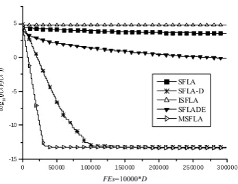
Figure 10. Convergence Graph for f9
0 50000 100000 150000 200000 250000 300000 0.8
1.0 1.2 1.4 1.6 1.8 2.0 2.2 2.4 2.6 2.8
lo
g10
(
f(
x
)
-f(
x
*))
FEs=10000*D
SFLA SFLA-D ISFLA SFLADE MSFLA
Figure 11. Convergence Graph for f10
V. CONCLUSION AND FUTURE WORK
In order to improve algorithm’s intensification ability, a dimension by dimension strategy is used to do fine grained search based on SFLA. The individual update equation is redesigned to maintain the same probability close to the best solution with the original algorithm. The experiment simulations, which were carried on ten different kinds of benchmark function optimization problems, indicate that iterative improvement strategy can improve the intensification ability of SFLA remarkably. The overall performance of SFLA-D is superior to or at least competitive with some other selected algorithms from literature.
In future study, we will apply the proposed algorithm to solve some real-world problems. We will also verify the improvement strategy for other intelligent optimization algorithm.
ACKNOWLEDGMENT
The authors wish to thank any anonymous reviewers for providing valuable comments to improve this paper. This work was sponsored by Nature Science Foundation of Fujian Province of P. R. China (Project No. 2013J01216).
APPENDIX A TEST FUNCTONS
Name Range Goal
Sphere [-100 100] 10-6 Rosenbrock [-30,30] 10-6
Ackley [-30,30] 10-6 Griewank [-600,600] 10-6
Rastrigin [-5.12,5.12] 10-6 Schwefel [-500 500] 10-6 Generalized Penalized 1 [-50 50] 10-6 Generalized Penalized 2 [-50 50] 10-6 Shifted Sphere [-100 100] 10-2 Shifted Rotated Rastrigin [-5 5] 10-2
REFERENCES
[1] M. M. Eusuff, K. E. Lansey, Optimization of water distribution network design using the shuffled frog leaping algorithm. J. Water Resour. Plann. Manage. vol. 129(3), pp.210-225, 2003.
[2] E. Elbeltagi, T. Hegazy, D. Grierson. A modified shuffled frog-leaping optimization algorithm: applications to project management. Struct Infrastruct E., vol. 3(1) , pp.53-60, 2007.
[3] G. Chung, K. Lansey. Application of the shuffled frog leaping algorithm for the optimization of a general large-scale water supply system. Water Resour. Manag., vol. 23(4) , pp.797-823, 2009.
[4] B. Amiri, M. Fathian, A. Maroosi. Application of Shuffled frog leaping algorithm clustering. Int. J. Adv. Manuf. Tech.,
vol. 45(1-2) , pp.199-209, 2009
[5] H. Gao, J. Cao. Membrane-inspired quantum shuffled frog leaping algorithm for spectrum allocation. J. Sys. Eng. Elec., vol. 23(5), pp. 679-688, 2012.
[6] J. Lin, Y.W. Zhong, J. Zhang. A Modified Discrete Shuffled Flog Leaping Algorithm for RNA Secondary Structure Prediction. Adv. in Control. Comm., pp. 591-599, 2012.
[7] A. Bhaduri. A clonal selection based shuffled frog leaping algorithm. Advance Computing Conference, IACC 2009.
IEEE International. IEEE, 2009, pp. 125-130.
[8] Z. Zhen, D. Wang, Y. Liu. Improved shuffled frog leaping algorithm for continuous optimization problem. Evolutionary Computation, 2009. CEC'09. IEEE Congress
on. IEEE, 2009, pp. 2992-2995.
[9] X. Li, J. Luo, M. R. Chen, et al. An improved shuffled frog-leaping algorithm with extremal optimization for continuous optimization. Inform. Sciences, vol. 192,
pp.143-151. 2012,
[10]J. P. Lou, M. R. Chen. Study on Trajectory and Convergence Analysis of Shuffled Frog Leaping Algorithm and Its Improved Algorithm. Signal Process. ,
vol. 26(9), pp.1428-1433, 2012.
[11]P. J. Zhao. Shuffled Frog Leaping Algorithm Based on differential disturbance. J. Comput. Appl., vol. 30(10), pp.
2575-2577, 2010.
[12]W. P. Ding, J. D. Wang, Z. J. Guan. Efficient Rough Attribute Reduction Based on Quantum Frog-Leaping Co-Evolution. Acta. Electronica. Sigica., vol. 39(11), pp.
2597-2603, 2011.
[13]X. D. Zhang, L. Zhao, C. R. Zou. An improved shuffled frog leaping algorithm for solving constrained optimization problems. J. Shan Dong University(Eng. Sci.), vol. 43(1),
pp. 1-8, 2013.
2005005, 2005.
[15]J. J. Liang, A. K. Qin, P. N. Suganthan, et al. Comprehensive learning particle swarm optimizer for global optimization of multimodal functions. IEEE T. Evolut. Comput., vol.10 (3), pp. 281-295,2006.
[16]Y.W. Shang, Y.H. Qiu. A note on the extended rosenbrock function. IEEE T. Evolut. Comput., vol. 14(1), pp. 119-126,
2006.
[17] E. Elbeltagi, T. Hegazy, D. Grierson. Comparison among five evolutionary-based optimization algorithms. Adv. Eng. inf. , vol. 19(1), pp.43-53, 2005.
Juan Lin is a lecturer at the College of
Computer and Information at the Fujian Agriculture and Forestry University, Fuzhou, China. She received her MS in bioinformatics from Fujian Agriculture and Forestry University in 2011. Her current research interests include computational intelligence and bioinformatics.
Yiwen Zhong is a Professor at the