A New-type Pi Calculus with Buffers and
Its Bisimulation
Hui Kang
College of Computer Science and Technology, Jilin University, Changchun, Jilin Province, China Email: [email protected]
Zhi Wang, Shuangshuang Zhang and Fang Mei
College of Computer Science and Technology, Jilin University, Changchun, Jilin Province, China Email: [email protected], [email protected], [email protected]
Abstract—According to the features of asynchronous inter-action in systems, a new-type Pi calculus with buffers — Buffer-Pi calculus is proposed, the new labelled transition system based on buffers is introduced, the enhanced de-scribing capability is shown to apply Buffer-Pi calculus to modeling with the concrete example of asynchronous inter-action, and the new behavior equivalence relations are de-fined, several propositions and properties of Buffer-Pi cal-culus are given. The study shows that compared with Pi calculus, Buffer-Pi calculus can provide more powerful support for asynchronous behavior modeling in systems.
Index Terms—asynchronous interaction, Buffer-Pi calculus, the labelled transition system with buffers, behavior equiv-alence relation
I. INTRODUCTION
In the past few decades, with the development of computer science and communications technology, in-teractive systems have become increasingly popular, and the way of computing has changed a lot from the tradi-tional sequential calculation [1][2] extended to the con-current computing with interaction [3][4] as the main feature, simultaneously both location [5-8] and mobility [9][10] are characterized as independent concepts in the formal model. Pi calculus [11] proposed by Robin Milner is a kind of process algebra method describing concur-rent interactive systems, whose basic entities are pro-cesses and names. The syntax and semantics of Pi calcu-lus can be found in the Reference [11-14], and they are not repeated here. Pi calculus is a computational model based on synchronization interactive pattern with a lack of asynchronous features. However, with the develop-ment of network technology, asynchronous communica-tion technology with Ajax [15][16] as the representative has become a mainstream, so it requires a corresponding formal method to describe and analyze systems with asynchronous features [17].
In previous work, there are two main methods to han-dle asynchronous interaction in the process algebra framework represented by Pi calculus: One method is to use the parallel operator instead of output prefix [18], for
example, X =a(m1).b(m2).c(m3).P represents sending the messages m1, m2, m3 in turn through the channels a, b and c, and then executing P (Here P means the remain-ing calculation of the process X). The above formula only reflects the sequential features of sending messages, but not asynchronous features of system interaction. Then the above formula can be changed into
P m c m b m a
X = ( 1)| ( 2)| ( 3)| , and in this formula asynchro-nous features are shown, while the messages cannot reach the other side of the interaction in turn. The other method is to send a message by constructing components such as a buffer [19]. In this case, the above formula can be shown as X = i('m).P , which indicates that the
buffer i' receives the output message m, and at the
same time P can be executed without waiting. These two methods both have advantages and disadvantages: The first method is simple, but the messages may reach without order; the second method is practical, but it is too complicated.
paper, The main work is as follows: (1) proposing a new-type of Pi calculus with buffers—Buffer-Pi calculus; (2) in the concept of buffers, putting forward a new la-belled transition system with buffers; (3) giving the new behavioral equivalence of Buffer-Pi calculus on the basis of (2); (4) the propositions and properties of Buffer-Pi calculus are given using the definition in (3).
II.THE SYNTAX OF BUFFER-PI CALCULUS, THE LABELLED TRANSITION SYSTEM WITH BUFFERS, AND EXTENDED
OPERATIONAL SEMANTICS
A. Basic Concepts
Before the syntax of Buffer-Pi calculus is given for-mally, the following basic concepts are offered at first.
Definition 1 Basic Type and Compound Type: As mentioned above, there are two kinds of basic entities in Pi calculus—processes and names. Names can represent channels, and one new channel can be transmitted by a known channel. Processes received can use the new channel to establish a connection, so the type of CHANNEL is introduced for these names. Names can also represent data information, such as integer, boolean
string and so on, therefore the type of VALUE is in-troduced for them. Therefore, the basic type
t
ˆ
can be defined as follows:VALUE CHANNEL tˆ::= |
Besides the basis type, the operators of type structure can be used to construct the compound type. For instance, Cartesian production
'
×
'
can be used to construct the type of dual. With the level structure of names intro-duced here, LAYERis defined as the operator of levelstructure. The type hierarchy consisting of LAYER and
sequence of all types can be defined now, such as: L
()), ()),
( (
(),LAYER LAYER LAYER LAYER LAYER
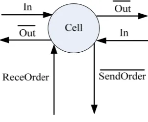
Definition 2 Buffer Cell: A buffer cell is a triple, Cell=(ident, type, port), where ident is the unique identi-fier of a buffer cell(the ident of cells in the buffer is buffer identifier and location index), the type is the entity type stored in buffer cells, and the port is used for buffer cells to interact with the outside, just as Fig. 1 shows:
Figure 1. The basic structure of a Cell
It can be seen from Fig. 1 that the Cell can complete the two-way transmission of information (inIn and Out ports). As a result of the symmetry of information trans-mission, this paper only makes formal description and
analysis of a single direction of information transmission without special instruction.
In order to facilitate the formal description of the Cell and system modeling below, some notations will be in-troduced. A(p1,L,pn) denotes a definition identifier
of the process, and (p1,L,pn)is its port parameter list. >
<c cn
port 1,L, indicates that processes can send or receive commands by port, and <c1,L,cn>is its com-mand parameter list. A(p1,L,pn)→port<c1,L,cn> is
the port action with its command parameter list when reaching the process A.
As for the Cell, there are the following ports:
In: receiving outside information, and storing it in the Cell.
Out: sending the information of the Cell to the out-side.
ceOrder
Re : receiving commands from the Sched-uler. When the Cell receives the command “RedayReceive” from the port ReceOrder, the port In will start to receive data; when receiving “ReadySend”, the port Out will start to send data.
SendOrder: the Cell sending commands to the
Sched-uler. When there is content stored in the Cell, the com-mand “CanSendData” will be sent, and the Scheduler will be told that the Cell is in the state that can sent data and will block the port In to receive data. When there is nothing in the Cell, the command “CanReceiveData” will be sent, and the Scheduler will be told the Cell is in the state that can receive data and will block the port
Out to send data.
The definition of Cell(In,Out,ReceOrder,SendOrder) is
given, and:
> <
> <
= ′
> <
′
> <
=
ceiveData Can
SendOrder Cell
Out
adySend ceOrder
l Cel
a CanSendDat SendOrder
l Cel In
ceive ady ceOrder
Cell
def def
Re .
. Re
Re .
. Re Re Re
a
a (1)
From the perspective of process algebra, the definition of the Cell is a process expression with certain action.
Definition 3 Buffer: It is an ordered set composed of the same type of buffer cells. A buffer is a triple. Buffer = (ident, type, n), where the ident is the unique identifier of buffer, the type means data type stored in buffer cells, and n indicates the current buffer size, whose structure can be expressed as follows:
} , , , , { :: )
( ( ) ( ) ( )
1 )
( n
n n
v n
n Cell Cell Cell
ident
type = L L (2)
The current buffer size n is also known as the length of the buffer, and it can be obtained by length(ident),
)
max(ident means the maximum capability that the buffer can apply, and type(ident) means the data type of the buffer. Here is an example of defining a buffer below. ( ) (n)
Buff
with the increase and decrease of buffer cells. (n) v Cell
means the vth Cell in the buffer with the size n.
The component Buffer in this paper is used in asyn-chronous interaction of the system. As stated in the in-troduction, sending or receiving asynchronous messages is directional and sequential, so the Buffer in the defini-tion is an ordered set, and the first Cell ( ( )
1
n
Cell ) in the Buffer is called the Header, the last Cell ( (n)
n Cell ) is
called the Tail.
In terms of the entity type stored in buffers, the buffer can be divided into the channel buffer (ChannelBuffer), the data buffer (ValueBuffer) and the composite buffer (CompoundBuffer). In addition, processes during the execution can create a buffer with several processes, and the type of interactive information may be CHANNEL or DATA, even there may be more complex compound type, so the set consisting of all kinds of buffers for the spe-cific process is named buffer set, denoted as BufferSet.
In order to distinguish synchronous or asynchronous interaction of the system, the port action between the processes is abstracted into two classes, one is the asyn-chronous port action, denoted as [port], and the other is the synchronous port action, denoted as <port>(Buffer-Pi calculus syntax will be described further in the follow-ing).
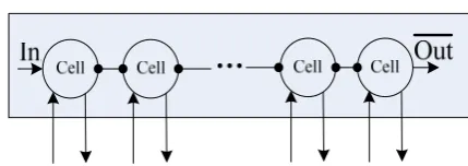
Definition 4 Buffer Chain: Intuitively, it links the right port (Out)of a cell to the left port(
In
) of the next cell, and adjacent cells are linked by port just as Fig. 2 shows. The below is the formal definition of a binary chain and brings in the link operator∩
:) } / { | } /
({ 1
1 +
+
∩ =
v v
def
v
v Cell newl l OutCell l InCell
Cell (3)
Figure 2. Weak equivalence chain structure of the Buffer
Fig. 2 shows the weak equivalence chain structure of the Buffer. The ports ReceOrder and SendOrder are
omitted and only a single direction of information trans-mission is given, but this does not affect the external function of the Buffer.
Since the topic of this paper is the component Buffer, so here the functional description of the Scheduler is only given, as shown in Fig. 3, where
a
v is the control interaction with the port ReceOrder of (n)v
Cell , and bv
is the control interaction with the port SendOrder of )
(n v
Cell . By means of the command interaction of the
Schedule and the Buffer, it ensures that the external ac-tion of the Buffer keeps coordinaac-tion and order.
Figure 3. The structure of the Scheduler
Proposition 1 64 74L4 84
n
n
Cell Cell
Buff()≈ ∩ ∩ (4) Proof: In the Reference [20] the similar property is given: it indicates that the buffer (n)
Buff independently composed of n cells is weak equivalent to the compo-nents linked by n cells. However, the cell structure pro-posed in this paper is different from that in the Reference [20]. The buffer cell in the Reference [20] is a simple process structure only with left and right port while the cell structure is refined in this paper. As the cell structure in this paper is extended on the basis of that in the Ref-erence [20], the property above can also be applied in this paper.
□
Moreover, in Fig. 2, the function ports of the Buffer do not change much compared with that in the Cell, and the information ports interacting with the outside does not increase(InandOut). Only the control ports
interact-ing with the Scheduler is changinteract-ing in the quantity with the variation of the buffer size (ReceOrderand
)
SendOrder . Therefore the formal definition of the
Buffer has no essential difference with the Cell, and it is omitted. Buff_Controller new(ReceOrder,SendOrder)(Buff|
def
=
)
Scheduler will be used as a whole in order to facilitate modeling.
The complementary actions of In and Out are de-fined as follows.
In order to interact with theBuff _Controller, the complementary actions of Inand Outare defined as follows:
) (name
In : It indicates the interactive mode of asyn-chronous output from processes to buffers. The parame-ter name means the information stored in the buffer successively according to the order of the process output. By executing in parallel with the process, it can interact with the Buff_Controller. Before asynchronous output in the process, the buffer must enter the state which can receive data, and can be operated through the buffer ex-pression associated with the evolutionary action. When processes have finished asynchronous output, new in-formation will be added to the tail of the parameter
name.
) (name
Out : It indicates the interactive mode of
through the buffer expression associated with the evolu-tionary action. When processes have finished asynchro-nous input, information which has been send will be de-leted from the header of the parameter name.
Definition 5 Buffer Partial Order and Buffer Equiva-lency: For the Buffer B1 and the Buffer B2, they are denoted as B1pB2, if type(B1) =type(B2) , and
) ( )
(B1 length B2
length ≤ .
For the Buffer B1 and the Buffer B2, they are
de-noted as B1 =B2, if B1 pB2 and B2 pB1.
Definition 6 BufferSet Partial Order and BufferSet Equivalency: For the two BufferSets BufferSet1 and
2
BufferSet owned by the processes P1 and P2, they are denoted as BufferSet1<BufferSet2 , if
| |
|
|BufferSet1 = BufferSet2 and to each element B1 in
1
BufferSet , there is a unique element B2 corresponding with, making B1 pB2 be true, and the contrary is also true.
For the two BufferSets BufferSet1 and BufferSet2 owned by the processes P1 and P2, they are denoted as
2 1 ˆ BufferSet
BufferSet = , if |BufferSet1|=|BufferSet2| and to each element B1 in BufferSet1, there is a unique elementB2corresponding with, making B1=B2 be true, and the contrary is also true.
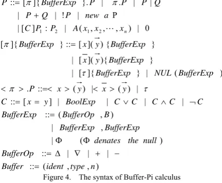
B. The Syntax of Buffer-Pi Calculus
For Buffer-Pi calculus, a crucial task is to determine how the system's dynamic execution semantics be asso-ciated with the Buffer’s creation, destruction and update, which comes true by Buffer’s operators, and Fig. 4 shows the complete syntax of Buffer-Pi calculus.
) , , ( ::
| | | ::
) (
|
, |
) , (
::
| |
| |
] [ ::
| ) ( | ) ( ::
.
) (
| } ]{
[ |
} ){
]( [ |
} {
) ]( [ :: } ]{
[
0 | ) , , , ( | : ] [ |
P |
! | |
| | . | }. ]{
[ ::
2 1 2 1
n type ident Buffer
BufferOp
null the denates
BufferExp BufferExp
B BufferOp BufferExp
C C C C C BoolExp y
x C
y x y x P
BufferExp NUL
BufferExp BufferExp y
x
BufferExp y
x BufferExp
x x x A P P C
a new P Q P
Q P P P BufferExp P
n
=
− + ∇ Δ =
Φ Φ =
¬ ∧ ∨
= =
> < > =< > <
= +
=
τ π
τ π
π π
L
Figure 4. The syntax of Buffer-Pi calculus
In Fig. 4, two prefix actions are defined, one is asyn-chronous interaction associated with the buffer expres-sion([π]{BufferExp}), and the other is synchronous interaction (<
π
>.P). π{BufferExp} introduces a special action NUL(BufferExp), which means to op-erate the buffer independently without the evolutiveac-tion of the system. Buffer operaac-tion implements a rela-tion of buffer conversion ℜ:BufferSet′×BufferOp ×B
t BufferSe ′′
→ , that is to say, the buffer set which exists in the current system and the buffer expression can iden-tify a new buffer set. In particular, there are four kinds of buffer operation in Buffer-Pi calculus, they are as fol-lows:
1 creation of buffers (Δ): create a new buffer, speci-fying the buffer type and the initial length n.
2 destruction of buffers (∇): remove the specified buffer from the BufferSet of the current process.
3 addition of buffer cells (+): add a new buffer cell to the Tail of a buffer.
4 deletion of buffer cells (-): delete the buffer cell from the Header of a buffer.
In order to facilitate the unified representation below, ]
[α signify the asynchronous action in the system asso-ciated with the buffer expression, that is to say
} ]{
[ ]
[α = π BufferExp , <α> signifies synchronous ac-tion in the system, and α signify the abstract action in the general sense. The key point of this paper is the properties of systems in asynchronous interaction, and synchronous action in the system is the same as basic Pi calculus, therefore in the case of no special instruction, the following discussions all aim at the asynchronous interaction.
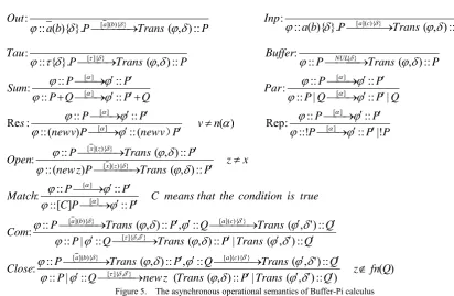
C. The Labelled Transition System with Buffers Based on the above definition, a new labelled transi-tion system is presented in this sectransi-tion—the labelled transition system with buffers.
Definition 7 the Labelled Transition System with Buffers: In the Buffer-Pi calculus, the labelled transition system with buffers ( , ,{⎯[⎯]{⎯BufferExp⎯⎯ }→
M
S π
})
|π∈M consists of the following elements: S is a two-tuple set consisting of processes and the BufferSet associated with it, M is the labelled set, while the transi-tion set is
{
⎯
{⎯
BufferExp⎯
⎯
}[⎯
π]→
}
⊆S× S,π ∈ M .In the labelled transition system with buffers, the tran-sition {BufferSet′}::P′⎯[⎯π]{⎯BufferExp⎯⎯ }→{BufferSet′′}
P′′
:: indicates that the current process P′ has the buffer set named BufferSet', and through implementing an asynchronous action [π] which is associated with the buffer expressionBufferExp, P′ is converted into P′′ with a buffer set namedBufferSe t′′. In order to con-veniently make a description of the Buffer-Pi calculus asynchronous operational semantics, the method Trans is defined strictly as follows:
⎪ ⎪ ⎩ ⎪⎪ ⎨ ⎧
′ =
ℜ
= ′
′′ →
× ′
null is BufferExp if
t BufferSe
B BufferOp BuferfExp
if
B BufferOp BuffSet
BufferExp t
BufferSe Trans
t BufferSe BufferExp
t BufferSe Trans
) , (
) , ,'
(
) ,
( :
) ( ) :: ) , ( | :: ) , ( ( :: | :: :: ) ' , ( :: , :: ) , ( :: : :: ) , ( | :: ) , ( :: | :: :: ) ' , ( :: , :: ) , ( :: : :: ] [ :: :: :: : :: ) , ( ) ( :: :: ) , ( :: : |! :: ::! :: :: : Rep ) ( ( :: ) ( :: :: :: : Re | :: | :: :: :: : :: :: :: :: : :: ) , ( :: : :: ) , ( }. { :: : } / { :: ) , ( }. ){ ( :: : :: ) , ( }. ){ ( :: : } , ]{ [ } ){ ]( [ } ){ ]( [ } , ]{ [ } ){ ]( [ } ){ ]( [ ] [ ] [ } ){ ]( [ } ){ ]( [ ] [ ] [ ] [ ] [ ] [ ] [ ] [ ] [ } { } ]{ [ } ){ ]( [ } ){ ]( [ Q fn z Q Trans P Trans z new Q P Q Trans Q P Trans P Close Q Trans P Trans Q P Q Trans Q P Trans P Com true is condition the that means C P P C P P Match x z P Trans P z new P Trans P Open P P P P P n v P v new P v new P P s Q P Q P P P Par Q P Q P P P Sum P Trans P Buffer P Trans P Tau b c P Trans P b a Inp P Trans P b a Out c a b a c a b a z x z x NUL c a b a ∉ ′ ′ ′ ′ ⎯ ⎯ ⎯ → ⎯ ′ ′ ′ ⎯ ⎯ ⎯ → ⎯ ′ ′ ⎯ ⎯ ⎯ → ⎯ ′ ′ ′ ′ ⎯ ⎯ ⎯ → ⎯ ′ ′ ′ ⎯ ⎯ ⎯ → ⎯ ′ ′ ⎯ ⎯ ⎯ → ⎯ ′ ′ ⎯→ ⎯ ′ ′ ⎯→ ⎯ ≠ ′ ⎯ ⎯ ⎯ → ⎯ ′ ⎯ ⎯ ⎯ → ⎯ ′ ′ ⎯→ ⎯ ′ ′ ⎯→ ⎯ ≠ ′ ′ ⎯→ ⎯ ′ ′ ⎯→ ⎯ ′ ′ ⎯→ ⎯ ′ ′ ⎯→ ⎯ + ′ ′ ⎯→ ⎯ + ′ ′ ⎯→ ⎯ ⎯ ⎯ ⎯ → ⎯ ⎯ ⎯ → ⎯ ⎯ ⎯ ⎯ → ⎯ ⎯ ⎯ ⎯ → ⎯ ′ ′ ′ ′ δ ϕ δ ϕ ϕ ϕ δ ϕ ϕ δ ϕ ϕ δ ϕ δ ϕ ϕ ϕ δ ϕ ϕ δ ϕ ϕ ϕ ϕ ϕ ϕ δ ϕ ϕ δ ϕ ϕ ϕ ϕ ϕ ϕ α ϕ ϕ ϕ ϕ ϕ ϕ ϕ ϕ ϕ ϕ ϕ ϕ δ ϕ ϕ δ ϕ δ τ ϕ δ ϕ δ ϕ δ ϕ δ ϕ δ δ τ δ δ δ δ τ δ δ α α δ δ α α α α α α α α δ δ τ δ δ )
Figure 5. The asynchronous operational semantics of Buffer-Pi calculus
D. The Extended Operational Semantics of Buffer-Pi calculus
Fig. 5 gives the asynchronous operational semantics of Buffer-Pi calculus, where
ϕ
andδ
respectively means BufferSet and BufferExp,ϕ
′ is the buffer set after the buffer operation associated with asynchronous action [α], and fn and bn respectively means the free name set and the bound name set.In Fig. 5, the asynchronous operational semantics of Buffer-Pi calculus is given, and the synchronous opera-tional semantics is the same as that of basic Pi calculus, which can be found in the Reference [11], here it isn’t repeated. It should be pointed out that the asynchronous operational semantics of Buffer-Pi calculus can not only do buffer operation through the buffer expression associ-ated with process action, such as Out, Inp and Tau, but also can do the direct operation to buffers through
). (BufferExp
NUL
E. The Modeling and Analysis of Processes with Asynchronous Interaction based on Buffer-Pi Calculus
As shown in Fig. 6, a simple example of processes with asynchronous interaction is given. The asynchro-nous messagesm1,m2 are passed on through the port α , and the synchronous message m3 is passed on through the port β. There is only one buffer with the type CHANNEL in the BufferSet between P and Q, but it explains the problem fully.
First of all, according to the basic Pi calculus, the formal description of the whole system can be made as follows:
Figure 6. Processes with asynchronous interaction based on Buffer
Q P System Q m m m Q P m m m P | ). ( ). ( ). ( ). ( ). ( ). ( 3 2 1 3 2 1 = ′ ′ ′ ′ = ′ = β α α β α α
After introducing the component Buffer, the system can be modeled by using Buffer-Pi calculus:
) | | _ ( :: :: ) | ( ) , (Re _ ). ( :: | ) , ( :: ). ( :: | ) , ( :: } , { ) ( 3 2 1 3 2 1 2 1 2 Q P Controller Buff Buff System Buff Scheduler Buff SendOrder ceOrder new Controller Buff Q m Buff m m out Q Buff P m Buff m m In P Buff m m Buff CHANNEL = = ′ > < = ′ > < = = β β
For the Buff in the above definition, when the process P needs to send the new information m4 to Q, the
transition of basic Pi calculus is
P
'
⎯
α⎯ →
(m⎯
4)P
′′
,} , , { )
(
) |
(
) ,
(Re _
) _
| | ). ( |
) , , ( ( :: ::
4 2 1 3
3
4 2 1 )}
, ){( ](
[ 4
m m m f Buf CHANNEL
Scheduler f
Buf
SendOrder ceOrder
new r Controlle Buff
r Controlle Buff
Q P m
m m m In f Buf System
Buff m Buff
= ′
′ =
′
′ ′′
> <
′ ⎯ ⎯ ⎯ ⎯
⎯ →
⎯ +
β
α
For the Buff, when the process Q receives the asyn-chronous message m1, the transition of the basic Pi
cal-culus is Q⎯⎯ →m⎯′ (m2). (m3).Q′
)
( 1 α α
α , the following
transition can be gained through applying Buffer-Pi cal-culus:
} { )
(
) |
(
) ,
(Re _
) _
| | ). (
| ) ( ( :: ::
2 1
3
2 )}
, ){( ]( [ 1
m f Buf CHANNEL
Scheduler f
Buf
SendOrder ceOrder
new r Controlle Buff
r Controlle Buff
P Q m
m Out f
Buf System
Buff m Buff
= ′
′ =
′
′ ′
> <
′ ⎯
⎯ ⎯ ⎯
⎯ →
⎯ ′ −
β
α
III. BUFFER BISIMULATION AND ITS PROPERTY ANALYSIS
Bisimulation equivalence is the core issue of process algebra. In basic Pi calculus, strong / weak bisimulation equivalence have been defined [11], while in Buffer-Pi calculus, the impact which buffer operations bring in need to be considered, since the component Buffer is in-troduced. So in this section the concept of bisimulation will be redefined on the basis of the labelled transition system with buffers defined above. To be convenient, the following symbols are given at first: ⇒ indicates a transition sequence composed of a number of actions that
are not visible (its length can be 0); ⇒α means ⇒→α ⇒,
where α is a visible action. ⇒αˆ means if
α
=τ
then=⇒
⇒αˆ ,and if
α
≠
τ
, then⇒
α=
⇒
αˆ
;
⇒
α means an action sequence with any length. A simplified representa-tion of processes in Buffer-Pi calculus is given below. For a process expression of basic Pi calculus P, using the asynchronous action prefix [α] and the synchronous action prefix <α>, the action of asynchronous and synchronous in the process P is distinguished. For exam-ple, P=α(m1).α(m2).β(m3).P′ is changed intoP m m
m
P=[α]( 1).[α]( 2).<β >( 3). ′.
Definition 8 Strong Mixed Buffer Bisimulation: the symmetric binary relation R in Buffer-Pi calculus is called strong mixed buffer bisimulation, if to
) :: (
) ::
(BufferSetP P RBufferSetQ Q , ⎯⎯→
α
P BufferSetP::
P
BufferSetP′:: ′, then there exists a Q′, which makes
) max(
)
max(BufferSetP′ = BufferSetQ′ , BufferSetP′=ˆ
′ Q
BufferSet ,and (BufferSet P ::P )R(BufferSet Q ::Q′) ′ ′
′ .
Definition 9 Weak Mixed Buffer Bisimulation: the symmetric binary relation R in Buffer-Pi calculus is
called weak mixed buffer bisimulation, if to
) :: (
) ::
(BufferSetP PR BufferSetQ Q , ⎯⎯→
α
P BufferSetP::
P
BufferSet P′:: ′ , then there exists a Q′ , which
makes max(BufferSetP′)=max(BufferSetQ′) , =
′ ˆ P BufferSet
′ Q
BufferSet , and (BufferSet P′::P′)R(BufferSet Q′::Q′).
In order to observe the impact of the buffers’ introduc-tion separately, the buffer is considered as an independent dimension of system description, and the system equiva-lence is described from the perspective of the component Buffer. In fact, abstracting out the buffer to make equiva-lence description can clearly describe the system's asyn-chronous interactivity, which contains the number and type of asynchronous interaction. Therefore it is quite necessary to do research on the asynchronous properties of interactive systems by defining the equivalence of buffers independently.
Definition 10 Buffer Simulation and Buffer Bisimulation: the symmetric binary relation R in Buff-er-Pi calculus is called buffer simulation, if
to (BufferSetP::P)
) :: (BufferSet Q
R Q , BufferSetP P BufferSetP P′
′ ⎯→
⎯ ::
:: α ,
then there exists a Q′, which makes max(BufferSetP′)
)
max( ′
= BufferSet Q ,
′ =
′
Q P BufferSet
BufferSet ˆ , and
) :: (
) ::
(BufferSet P P R BufferSet Q Q′ ′ ′
′ .
The symmetric binary relation R in Buffer-Pi calculus is called buffer bisimulation, only if R and its inverse
1
−
R both are buffer simulation.
Proposition 2 Buffer bisimulation is a kind of equiva-lence relation.
Proof: The reflexivity is obviously true. To prove the symmetry, it needs to prove that if the relation R is buffer bisimulation, then its inverse
R
−1 must be buffer bisimulation. From the definition of buffer bisimulation, it is obvious; For the transitivity, it must prove that if1
Rand R2both are buffer bisimulation, then their
com-posite relation is R1R2 ={(BufferSet p :: p,BufferSet r ::r)
}
|∃q pR1qandqR2r is also buffer bisimulation. It only needs to be enough to verify that R1R2 is buffer simula-tion. Suppose (BufferSetp::p,BufferSetr::r)∈R1R2 and BufferSetp::p⎯⎯→BufferSetp′::p′
α . Because there
exists
q
to meet (BufferSetp::p)R1(BufferSetq::q) and (BufferSetq::q)R2(BufferSetr::r), then also existsq
′
, which makes BufferSetq::q⇒BufferSetq′::q′μ
,
) max(
)
max(BufferSetp′ = BufferSetq′ , BufferSetp′ =ˆ ′
q
BufferSet and(BufferSet p ::p)R(BufferSetq ::q′)
′ ′
′ , so
there also exists an r′ , which makes
r BufferSet r
BufferSetr :: ⇒ r′:: ′ μ
)
max( ′
= BufferSetr ,
′ =
′
r q BufferSet
BufferSet ˆ
and (BufferSet q′::q′)R2(BufferSet r′::r′) and, so
2 1
) :: ,
::
(BufferSetp′ p′BufferSetr′ r′ ∈RR , therefore it
verify that R1R2 is buffer simulation. □ Proposition 3 If the process P and Q with buffers are
strong mixed buffer bisimulation or weak mixed buffer bisimulation, and then they must be buffer bisimulation.
Proof: From the definition of mixed buffer bisimulation and buffer bisimulation it can be obtained
directly. Proposition 3 has proved that the buffer bisimulation is
a looser equivalence relation relative to strong/weak mixed buffer bisimulation, which reflects the simulation of buffer state equivalent during the process evolution.
If there are processes P, Q and R, and there is a buffer BufferP between P and R, and a buffer BufferQ be-tween Q and R, when type(BufferP)=type(BufferQ)
and max(BufferP)=max(BufferQ ), it can be said that
P and Q have the same asynchronous processing capabil-ity of the same type, which is denoted as P Q
R
◊ . When type(BufferP)=type(BufferQ) and max(BufferP)
) max(BufferQ
> , it shows that P has a stronger asyn-chronous processing capability than Q, which is denoted as P Q
R
> .
Property 1 If P Q
R
◊ andtype(BufferP)=type(BufferQ)
CHANNEL
= , then P and Q have the same asynchronous structure converting capability.
Property 2 If P Q
R
◊ andtype(BufferP)=type(BufferQ)
DATA
= , then P and Q have the same asynchronous basic data transferring capability.
Property 1 and Property 2 give a standard to judge asynchronous processing capability of the specified cesses, which makes the processes’ asynchronous pro-cessing capability quantified and typed.
IV. SUMMARY
A. Analysis of Asynchronous Processing Capability In fact, in the Reference [18][19], the processing ap-proaches of asynchronous behavior are simply given, and their properties are not systematically discussed. Property 1 and Property 2 show the quantified standard of asyn-chronous processing capability in the system. For exam-ple, the process P with asynchronous behavior, the pro-cess expression in the form of Pi calculus is defined as follows:
) ( ). ( | ) ( ). ( ). ( | )
(x b y a y y u a z z v b
P=
where x is a name with the type CHANNEL of asyn-chronous features, and other free names is of synasyn-chronous features. Applying the methods of the Reference [18][19], asynchronous behavior of the process P isn’t presented, but using the Buffer-Pi calculus, it can be expressed as follows:
) ( ). ( | ) ( ). ( ). ( | )
( x b y a y y u a z z v b
P= < >
It can be seen that there are no subject names to ports of asynchronous features in the above formula. Therefore, for the current process P, it doesn’t need the component buffer. When the process P proceeds the further action, it is changed intop′=<x>(u)|<x>(v), where there is the asynchronous port x on two subject positions. It illus-trates at least the process P needs a buffer of
2 )
max(BufferP = in order to take full advantage of the
asynchronous processing capability of the process P.
B. Conclusion and Future Research
In this paper, according to the asynchronous features of interaction systems, a new-type Pi calculus with buff-ers—Buffer-Pi calculus is proposed on the basis of basic Pi calculus, the labelled transition system with buffers is defined, the Buffer-Pi calculus is applied to make a for-mal description of specific asynchronous processes with asynchronous interaction, and it is shown that the ex-tended Buffer-Pi strengthens the capability to describe system asynchronous behavior, and then the new behav-ior equivalence relations are proposed between the pro-cesses, and in the end several propositions and properties of the Buffer-Pi calculus are given.
On the basis of the above research, the future work in-cludes further extending typed bisimulation and comple-tion of scheduler model.
REFERENCES
[1] H. P. Barendregt, “The Lambda Calculus, Its Syntax and
Semantics,” North Holland, Revised edition, 1985.
[2] C. A. R. Hoare, “Communicating Sequential Processes,”
Communication of the ACM, vol. 21, no. 8, 1978.
[3] U. Montanari and M. Pistore, “Concurrent Semantics for
the Pi calculus,” In: Proceedings of MFPS’95, Electronic Notes in Theoretical Computer Science, vol. 1, pp. 411-429, 1995.
[4] R. Milner, “Communication and Concurrency,”
Pren-tice-Hall, 1989, in press.
[5] R. M. Amadio, “An asynchronous Model of Locality,
Failure, and Process Mobility,” In: COORDINATION97, Springer LNCS vol. 1282, pp. 374–391, 1997.
[6] R. Devillers, H. Klaudel, M. Koutny and F. Pommereau,
“Asynchronous Box Calculus,” Fundamenta Informaticae, vol. 54, no. 4, pp. 295-344, 2003.
[7] E. Best, R. Devillers and J. G. Hall, “The Box Calculus: a
New Causal Algebra with Multi-label Communication,” Advances in Petri Nets 1992, vol. 609, pp. 21-69, 1992.
[8] S. Davide, “Locality and interleaving semantics in Pi
cal-culus for mobile processes,” Theoretical Computer Science, vol. 155, pp. 39-83, 1996.
[9] J. E. White, “Mobile Agents,” MIT Press Cambridge, 1997,
in press.
[10]J. C. M. Baeten and W. P. Weijland, “Process Algebra,” Cambridge University Press, 1991, in press.
[11]R. Milner, J. Parrow and D. Walker, “A calculus of mobile
processes part I/II,” Journal of Information and Computa-tion, vol. 100, no.1, pp.1-77, 1992.
[12]M. Boreale and D. Sangiorgi, “A fully abstract semantics
of causality in the Pi calculus,” Technical Report ECS-LFCS-94-297, 1994.
[14]B. Victor, “The Mobility Workbench User’s Guider: Polyadic version 3.122,” Department of Information Technology, Uppsala University, 1995.
[15]J. G. Jesse, “Ajax: A New Approach to Web
Applica-tions,”www.adaptivepath.com/publications/essays/archives /000385.php.
[16]C. Gross, “Ajax Patterns and Best Practices,” Apress, 2006, in press.
[17]H. Klaudel and F. Pommereau, “Asynchronous links in the
PBC and M-nets,” In: Proceedings of ASIAN’99, Springer LNCS vol. 1742, pp. 190-200, 1999.
[18]K. Honda and M. Tokoro, “An Object Calculus for
Asyn-chronous Communication,” In: The 5th European Confer-ence on Object-Oriented Programming, Springer LNCS vol. 512, pp. 133–147, 1991.
[19]M. Dam, “Proof Systems for Pi-Calculus Logics”, Oxford
University Press, 2001, in press.
[20]R. Milner, “Communication and Mobile Systems: The
Pi-Calculus,” Cambridge University Press, 1999, in press.
Hui Kang (1967- ). Female, Han Dynasty, Changchun, Jilin
Province, China, College of Computer Science and Technology in Jilin University. Vice Professor, Research Field: IT Services and Network management.
Zhi Wang (1986- ). Male, Han Dynasty, Changchun, Jilin Province, China, College of Computer Science and Technology in Jilin University. Research Field: IT Services and Network management.
Shuangshuang Zhang (1989- ). Female, Han Dynasty,
Changchun, Jilin Province, China, College of Computer Science and Technology in Jilin University. Research Field: IT Services and Network management.
Fang Mei (1977- ) Female, Changchun, Jilin Province, China,