R E S E A R C H
Open Access
A general deep learning framework for
network reconstruction and dynamics
learning
Zhang Zhang
1, Yi Zhao
3, Jing Liu
1, Shuo Wang
2, Ruyi Tao
4, Ruyue Xin
1and Jiang Zhang
1**Correspondence: [email protected] 1School of Systems Science, Beijing Normal University, 100875 Beijing, People’s Republic of China Full list of author information is available at the end of the article
Abstract
Many complex processes can be viewed as dynamical systems on networks. However, in real cases, only the performances of the system are known, the network structure and the dynamical rules are not observed. Therefore, recovering latent network structure and dynamics from observed time series data are important tasks because it may help us to open the black box, and even to build up the model of a complex system automatically. Although this problem hosts a wealth of potential applications in biology, earth science, and epidemics etc., conventional methods have limitations. In this work, we introduce a new framework, Gumbel Graph Network (GGN), which is a model-free, data-driven deep learning framework to accomplish the reconstruction of both network connections and the dynamics on it. Our model consists of two jointly trained parts: a network generator that generating a discrete network with the Gumbel Softmax technique; and a dynamics learner that utilizing the generated network and one-step trajectory value to predict the states in future steps. We exhibit the
universality of our framework on different kinds of time-series data: with the same structure, our model can be trained to accurately recover the network structure and predict future states on continuous, discrete, and binary dynamics, and outperforms competing network reconstruction methods.
Keywords: Network reconstruction, Dynamics learning, Graph network
Introduction
Many complex processes can be viewed as dynamical systems on an underlying network structure. Network with the dynamics on it is a powerful approach for modeling a wide range of phenomena in real-world systems, where the elements are regarded as nodes and the interactions as edges (Albert and Barabási2002; Strogatz2001; Newman2003). One particular interest in the field of network science is the interplay between the network topology and its dynamics(Boccaletti et al.2006). Much attention has been paid on how collective dynamics on networks are determined by the topology of graph. However, in real cases, only the performances, i.e., the time series of nodes states are observed, but the network structure and the dynamical rules are not known. Thus, the inverse problems, i.e., inferring network topology and dynamical rules based on the observed dynamics data, is more significant. This may pave a new way to detect the internal structure of a system
according to its behaviors. Furthermore, it can help us to build up the dynamical model of a complex system according to the observed performance automatically.
For example, inferring gene regulatory networks from expression data can help us to identify the major genes and reveal the functional properties of genetic networks(Gardner et al. 2003); in the study of climate changes, network reconstruction may help us to reveal the atmospheric teleconnection patterns and understand their underlying mecha-nisms(Boers et al.2019); it can also find applications in reconstructing epidemic spreading processes in social networks, which is essential to identifying the source and preventing further spreading(Shen et al.2014). Furthermore, if not only the network structure but also the dynamics can be learned very well for these systems, surrogate models of the original problems can be obtained, on which, many experiments that are hard to imple-ment on the original systems can be operated. Another potential application is automated machine learning (AutoML)(Feurer et al.2015; Quanming et al.2018). At present, the main research problem of Neural Architecture Search(NAS), a sub-area of AutoML, is to find the optimal neural network architecture in a space by the search strategy, and it is essentially a network reconstruction problem, in which the optimal neural network and the dynamical rules on it can be learned according to the observed training samples as time series. In a word, reconstructions of network and dynamical rules are pivotal to a wide span of applications.
A considerable amount of methods have been proposed for reconstructing network from time series data. One class of them is based on the method of statistical inference such as Granger causality(Quinn et al.2011; Brovelli et al.2004), and correlation measure-ments(Stuart et al.2003; Eguiluz et al.2005; Barzel and Barabási2013). These methods, however, can usually discover functional connectivity and may fail to reveal structural connection (Feizi et al.2013). This means that in the reconstructed system, strongly cor-related areas in function need to be also directly connected in structure. Nevertheless this requirement is seldom satisfied in many real-world systems like brain (Park and Friston 2013) and climate systems (Boers et al.2019). Another class of methods were developed for reconstructing structural connections directly under certain assumptions. For exam-ple, methods such as driving response(Timme2007) or compressed sensing(Wang et al. 2011; Wang et al.2011; Wang et al.2011; Shen et al.2014) either require the functional form of the differential equations, or the target specific dynamics, or the sparsity of time series data. Although a model-free framework presented by Casadiego et al.(Casadiego et al.2017) do not have these limitations, it can only be applied to dynamical systems with continuous variables so that the derivatives can be calculated. Thus, a general framework for reconstructing network topology and learning dynamics from the time series data of various types of dynamics, including continuous, discrete and binary ones, is necessary.
2018), and spatial-temporal forecasting (Jain et al.2016; Li et al.2017; Yu et al.2017; Yan et al.2018). Recently, the topic of recovering interactions and predicting physical dynamics under given interaction networks has attracted much attention. A most used approach is introduced by Battaglia et al. (Battaglia et al.2016), representing particles as nodes and interactions as edges, then reconstruct the trajectories in a inference process on the given graph. However, most of the works in this field have focused on physi-cal reasoning task while few dedicate to solving the inverse problem of network science: revealing network topology from observed dynamics. Some related works (Watters et al. 2017; Guttenberg et al.2016) attempted to infer implicit interaction of the system to help with the state prediction via observation. But they did not specify the implicit interaction as the network topology of the system, therefore the network reconstruction task remains ignored. Of all literature as we known, only NRI (Neural Relational Inference) model(Kipf et al.2018) is working on this goal. Nevertheless, only a few continuous dynamics such as spring model and Kuramoto model are studied, and discrete processes were never con-sidered. So in the rest of this article, we will take NRI as one of our baselines and will be compared against our own model.
In this work we introduce Gumbel Graph Network (GGN), a model-free, data-driven method that can simultaneously reconstruct network topology and perform dynamics prediction from time series data of node states. It is able to attain high accuracy on both tasks under various dynamical systems, as well as multiple types of network topol-ogy. We first introduce our architecture which is called Gumbel Graph Networks in “GGN architecture” section and then give a brief overview of our experiments on three typical dynamics in “Experiments” section. In “Results” section, we show our results. Finally, some concluding remarks and discussions are given in “Conclusion” section.
GGN architecture Problem overview
The goal of our Gumbel Graph Network is to reconstruct the interaction graph and simulate the dynamics from the observational data ofNinteracting objects.
Typically, we assume that the system dynamics that we are interested can be described by a differential equationdX/dt = ψ(Xt,A)or the discrete iterationXt = ψ(Xt−1,A),
whereXt = (X1t, ...,XtN)denotes the states ofN objects at timet, andXiis the state of
the objecti.ψis the dynamical function, andAis the adjacency matrix of an unweighted directed graph. However,ψandAare unknown for us, and they will be inferred or recon-structed from a segment of time series data, i.e.,X=(Xt, ...,Xt+P), wherePis the number of prediction steps.
Thus, our algorithm aims to learn the network structure (Specifically, the adjacency matrix) and the dynamical modelψsimultaneously in an unsupervised way.
Framework
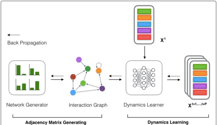
Fig. 1Basic structure of GGN. Our framework contains two main parts. First, the Adjacency Matrix is generated by the Network Generator via Gumbel softmax sampling; then the adjacency matrix andXt(node state at timet) are fed to Dynamics Learner to predict the node state in futurePtime step. The
back-propagation process runs back through all the computations
The Network Generator module uses the Gumbel softmax trick(Jang et al.2016) to generate the adjacency matrix. Details are explained in subsection 3. The goal of the Dynamics Learner is to map the features of all nodes from timetto timet+1 through generated adjacency matrix. Similar to NRI’s design(Kipf et al.2018), our GNN comprises of 4 mapping processes between nodes and edges, which can be accomplished through MLP, CNN or RNN module. In this article, we use MLP. Details are further explained in subsection 4. To learn the complex non-linear process, we use Graph Neural Network instead of Graph Convolutional Network(Kipf and Welling2016), since the latter does not consider the nonlinear coupling between nodes while sometimes it exists (for example, Kuramoto model).
The complexity on time and space are bothO(N2).
Network generator
One of the difficulties for reconstructing a network from the data is the discreteness of the graph, such that the back-propagation technique, which is widely used in differential functions, cannot be applied.
To conquer this problem, we apply Gumbel-softmax trick (Jang et al.2016) to recon-struct the adjacency matrix of the network directly. This technique simulates the sampling process from a discrete distribution by a continuous function such that the distributions generated from the sampling processes in real or simulation are identical. In this way, the simulated process allows for back-propagation because it is differentiable.
Network generator is a parameterized module to generate adjacency matrix. Specifi-cally, for a network ofNnodes, it uses aN×N parameterized matrix to determine the
N×Nelements in the adjacency matrixA, withαijdenoting the probability thatAijtakes
Specifically, the method to generate an adjacency matrix is shown below
Aij=
exp((log(αij)+ξij)/τ)
exp((log(αij)+ξij)/τ)+exp((log(1−αij)+ξij)/τ)
, (1)
whereξijs andξijs are i.i.d. random numbers following the gumbel distribution(Nadarajah
and Kotz2004). This calculation uses a continuous function with random noise to sim-ulate a discontinuous sampling process. And the temperature parameterτ adjusts the sharpness of the output distribution. Whenτ →0,Aijwill take 1 with probabilityαijand
0 with probability 1−αij.
Sinceαijs are all trainable parameters, they can be adjusted according to the back
prop-agation algorithm. Thanks to the features of Gumbel-softmax trick (Jang et al.2016), the gradient information can be back propagated through the whole computation graph although the process of sampling random numbers is non-differentiable.
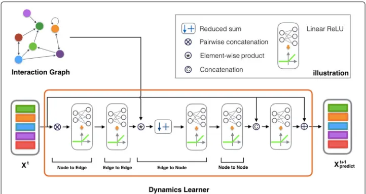
Dynamics learner
Learning with graph-structured data is a hot topic in deep learning research areas. Recently, Graph networks (GNs) (Battaglia et al.2018) have been widely investigated and have achieved compelling performance in node classification, link prediction, etc. In gen-eral, a GN uses the graph structureAandXt, which denotes features of all nodes at time
t, as its input to learn the representation of each node. Specifically, the graph informa-tion used here is the adjacency matrix constructed by the generator. The whole dynamics learner can be presented as a function:
Xpredictt =f(Xt−1,A) (2)
WhereXt is the state vector of allNnodes at time step t, Ais the adjacency matrix constructed by the network generator. Similar to the work (Kipf et al.2018), we realized this function through four mappings operating in succession: Node to Edge, Edge to Edge, Edge to Node and Node to Node, as shown below. Details are explained in the caption of Fig.2.
He1t−1=fv→e(Xt−1⊗(Xt−1)T) (3)
He2t−1=fe(He1t−1) (4)
Hv1t =fe→v(A∗He2t−1) (5)
Hv2t =fv(Hv1t ) (6)
Where,H.are hidden layers, Operation⊗is pair-wised concatenation, represented by
the formulav⊗v= vi,vj
N×N, resulting in a matrix where each element is a node
pair. The operation is similar to the Kronecker Product except that we replace the internal multiplication with concatenation. Element-wised product * of Adjacency matrix and the result of Edge to Edge mapping sets elements 0 if there is no connection between two nodes and Reduced sum operation will aggregate edge information to the node. The two trainable mapping functionsfe→vandfv→eare represented by neural networks.
Finally, we introduce skip-connection in ResNet (He et al.2015) to improve the gradient flow through the network, which enhances the performance of the Dynamics Learner.Xt
denotes the nodes’ states at timet.foutputis another MLP. This process can be presented
as a function
Xtpredict=foutput(Xt−1,Hv2t
)+Xt−1 (7)
Where [., .] denotes the concatenation operator, note that this operation, as well as the skip-connection trick are optional. We use these method only in experiments on Kuramoto. To make multi-step predictions, we feed in the output states and reiterate until we get the prediction sequenceXpredict = (Xpredict1 , ...,XpredictT ). Then we back propagate
the loss between model prediction and the ground truth.
Training
Having introduced all the components, we now present the training process as algorithm below. In the training process, we feed one step trajectory value:Xtas its input , and their
succeeding states, namely(Xt+1, ...,Xt+P)as the targets.
The dynamics learner and the network generator are altering optimized in each epoch. We first optimize the dynamics learner forSdrounds with the network generator fixed,
back propagating the loss to the dynamics learner in each round. Then the network gen-erator is trained with the same loss function as the dynamics learner forSn rounds. In
Algorithm 1:Gumbel Graph Network, GGN
P←Length of Prediction Steps;
Sn←Network Generator Train Steps;
Sd←Dynamics Learner Train Steps;
lr←Learning Rate;
Input:X= {X0,X1, ...,XP}
# Initialization: Initialize:
Network Generator parametersα; Dynamics Learner parametersθ; # Training:
foreach epochdo
A←Gumbel Generator(α); # Train Dynamics Learner;
form=1, ...,Sndo
X0predict←X0;
fort=1, ...,Pdo
Xpredictt ←Dynamics Learner(A,Xpredictt−1 ,θ);
end
loss←Compute Loss({X1, ...,XP},{X1predict, ...,XpredictP }); δθ ←BackPropagation;
θ ←θ−lr∗δθ;
end
# Train Network Generator;
forn=1, ...,Sddo
A←Gumbel Generator(α);
X0predict←X0;
fort=1, ...,Pdo
Xpredictt ←Dynamics Learner(A,Xpredictt−1 ,θ);
end
loss←Compute Loss({X1, ...,XP},{X1predict, ...,XpredictP }); δα←BackPropagation;
α←α−lr∗δα;
end end
Output:A,Xpredict = {Xpredict1 , ...,XpredictP }
In practice,SdandSnvary case by case. Although we chose them mainly through
hyper-parameter tuning, there is a general observation that the more complex the dynamics is, the largerSdit requires. For example, for Boolean Network model mentioned below,
Experiments An example
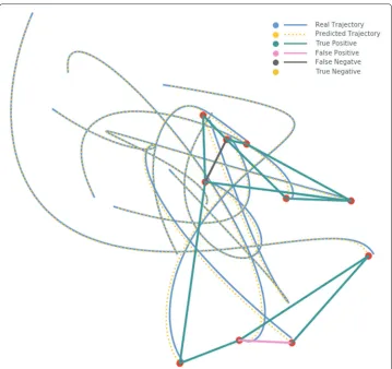
At first, we will show how GGN works and in what accuracy, we use a 10-body mass-spring interaction system as an example. Suppose in a two-dimensional plane, there are 10 masses linked each other by springs, and the connection density is 0.2. The masses can move according to the spring dynamics if the initial positions and velocities are given. And we will use the data of the position and velocity of each particle generated by the simulation to reconstruct their connections and predict their future positions.
In this experiment, we setSn =5 andSd =50, and use 5k training samples,1k
valida-tion samples and 1k test samples with each sample containing 3-steps trajectory of each mass. In each sample, one initial condition is adopted. The result shows that GGN can reconstruct the adjacency matrix with 97.8% accuracy, and can predict the next step posi-tions with a fairly small error 2.97∗10−5. Figure3visualizes the trajectories of simulation model and predictions.
It can be seen that GGN model can reconstruct the many-body problem in two-dimensional plane with high accuracy, and it can predict the node state in the future time accurately.
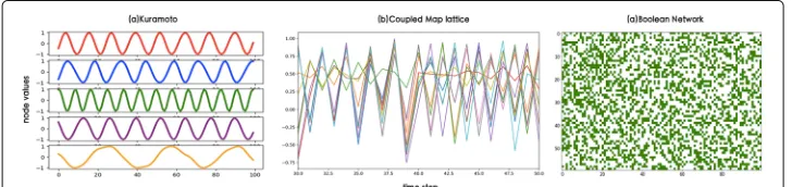
Experiments on simulated models
To systematically test the power of GGN, we experimented it on three types of simulated models: Boolean Network (Kauffman1969), Kuramoto (Kuramoto1975), and Coupled Map Lattice (Kaneko1992; 1989), which exhibit binary, continuous, and discrete tra-jectories, respectively. A schematic diagram of these systems is shown in Fig. 4. Here we attempt to train our model to learn the dynamics and reconstruct the interactions between particles, or the adjacency matrices, under all three circumstances.
Furthermore, we test the performance of GGN on different parameters with three main experiments: one concerns different net size and different level of chaos (subsection 3.1); one features different type of network topology (subsection 3.2), and one studies the rela-tionship between data size and accuracy (subsection 3.3). Our full code implementations are as shown on Github [https://github.com/bnusss/GGN].
Boolean network
Boolean Network is a widely studied model that is often used to model gene regulatory networks. In Boolean Network system, every variable has a possible value of 0 or 1 and a Boolean function is assigned to the node. The function takes the states of its neighbors as inputs and returns a binary value determining the state of the current node.
In simulation. We set the structure of the network as a directed graph with the degree of each node asK, and differentKdetermines whether the network will evolve chaoti-cally or non-chaotichaoti-cally. All nodes follow the same randomly generated table of dynamical rules. The training data we generated contains 5k pairs of state transition sequences. Meanwhile, we simulated 1k validation set and 1k test set.
Kuramoto model
The Kuramoto model (Kuramoto1975) is a nonlinear system of phase-coupled oscillators, and it is often used to describe synchronization. Specifically, we study the system
dφi
dt =ωi+k
j=i
Aijsin(φi−φj) (8)
Whereωi are intrinsic frequencies sampled from a given distributiong(ω), and here
we use a uniform distribution on [ 1, 10);kis the coupling strength;Aij ∈ {0, 1}are the
elements ofN × N adjacency matrix, and for undirected random networks we study,
Aij = Aji. The Kuramoto network have two types of dynamics, synchronized and
non-synchronized. According to studies by Restrepo et. al (Restrepo et al.2005), the transition from coherence to incoherence can be captured by a critical coupling strengthkc=k0/λ,
wherek0 = 2/πg(m), withmbeing the symmetric center ofg(ω), andλis the largest
eigenvalue of the adjacent matrix. The network synchronizes ifk>kc, and otherwise fails
to synchronize. We simulate and study both coherent and incoherent cases.
For simulation, we solve the 1D differential equation with 4th-order Runge-Kutta method with a step size of 0.01. Our training sets include 5k samplings, validation set 1k, and test set 1k, each sampling coversdφi/dtand sin(φi)in 10 time-steps.
Coupled map lattice
Coupled map lattices represent a dynamical model with discrete time and continuous state variables(Kaneko1992; 1989),it is widely used to study the chaotic dynamics of spatially extended systems. The model is originally defined on a chain with a periodic boundary condition but can be easily extended to any type of topology:
xt+1(i)=(1−s)f(xt(i))+
s
deg(i)
j∈neighbor(i)
f(xt(j)), (9)
where s is the coupling constant and deg(i) is the degree of node i. We choose the following logistic map function:
f(x)=λx(1−x). (10) We simulatedN ∈ {10, 30}coupled map lattices with initial statesx0(i)sampling
uni-formly from [ 0, 1] for random regular graphs. Notice that when setting coupling constant
s =0, the system reduces toNindependent logistic map. The training sets also include 5k samplings, 1k validation set, and 1k test set, each sampling coversxiin 10 time-steps.
Results
In each experiment listed below, we set the hyper-parametersSnandSd of the Boolean
Network model to 20 and 10, respectively, while in Coupled Map Lattice model and Kuramoto model they are 5 and 30. In Coupled Map Lattice model and Kuramoto model, the prediction stepsPis 9, which means that the current state is used to predict the node state of the next 9 time steps, while in the Boolean Network, it is set to 1. In all the experi-ments, we’ve set the hidden size in all the MLP networks of the dynamics learner module of the GGN model to 256. All the presented results are the mean value over five times of repeated experiments. The horizontal lines: “-” in the table indicates that the amount of data exceeds the model processing limitation, the model becomes so unstable that outputs may present as “nan” during training.
We compare our model with following baseline algorithms:
• NRI(Neural Relational Inference Model) is able to reconstruct the underlying network structure and predict the node state in future time steps simultaneously by observing the node state sequence. We compare our model against it in both tasks. Here we use settings similar to that in Kipf’s original paper(Kipf et al.2018): all our experiments use MLP decoders, and with the Kuramoto model, we use CNN encoder and other models the MLP encoder.
We use the following indicators to evaluate the results of the experiments:
• TPR(true positive rate) measures the proportion of positive instances that are correctly identified. We consider 1 in the adjacency matrix as a positive element, whereas 0 as a negative one.
• FPR(false positive rate) computes the proportion of negative instances that are incorrectly identified in the adjacency matrix generated.
• MSE(mean square error) measures the average of the squares of the errors, that is the average squared difference between the estimated values and data. The MSE we showed below is the average mean square error of nextP time steps.
• ACC(net)is the proportion of correctly identified elements of the Adjacency Matrix.
• ACC(dyn), In our experiment on the Boolean Network, we use indices ACC(dyn) to measure the proportion of nodes whose states are predicted accurately in the next time step.
Experiments with different dynamics
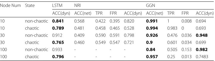
In our experiments, we set the network topology of a Boolean Network as a directed graph, with the indegree of each node beingk, andkdetermines whether the system is chaotic or not. For all systems, we setk =2 for non-chaotic cases; and for systems with 10, 30, 100 nodes,kis set to 7, 5 and 4, respectively, to obtain chaotic dynamics. As shown in Table1, the GGN model recovers the ground-truth interaction graph with an accuracy significantly higher than competing method, and the recovery rate in non-chaotic regimes is better than those in chaotic regime.
Here we presented our results obtained on coupled map lattice model in Table2. In our experiments, the network topology is random 4-regular graph, and we set coupling constants= 0.2 fixed. Becauser≈3.56995 is the onset of chaos in the logistic map, we choser = 3.5 andr = 3.6 to represent non-chaotic and chaotic dynamics respectively. For a random 4-regular graph with 10 nodes, our GGN model has obtained approximately 100% accuracy in the task of network reconstruction. For a system with 30 nodes, it is still able to achieve a high accuracy and the performance obtained on non-chaotic dynamics is better than that on chaotic dynamics.
Table 1Results with Boolean Network
Node Num State LSTM NRI GGN
ACC(dyn) ACC(net) TPR FPR ACC(dyn) ACC(net) TPR FPR ACC(dyn)
10 non-chaotic 0.841 0.568 0.422 0.395 0.820 0.991 1 0.008 0.694
10 chaotic 0.789 0.481 0.458 0.465 0.528 0.994 0.983 0 0.693
30 non-chaotic 0.912 0.409 0.590 0.591 0.798 0.926 0.476 0.036 0.948
30 chaotic 0.765 0.460 0.549 0.547 0.721 0.9 0.601 0.034 0.699
100 non-chaotic 0.933 - - - - 0.84 0.505 0.153 0.982
100 chaotic 0.796 - - - - 0.957 0.25 0.013 0.7483
Table 2Results with CML model
Node Num State LSTM NRI GGN
MSE ACC TPR FPR MSE ACC TPR FPR MSE
10 non-chaotic 1.92e-2 0.531 0.446 0.588 1.69e-4 1 1 0 5.63e-6
10 chaotic 2.54e-2 0.547 0.459 0.605 4.04e-4 0.993 1 0.013 3.24e-5
30 non-chaotic 4.11e-2 - - - - 1 1 0 3.29e-6
30 chaotic 5.03e-2 - - - - 0.999 1 0.0017 3.41e-6
The bold text represented the best results of a series of experiments
In the experiment concerning Kuramoto Model, we used Erdos-Renyi random graph with a connection possibility of 0.5. As the onset of synchronization is atk = kc(in our
cases,kc = 1.20 for 10 nodes system andkc = 0.41 for 30 nodes system), we chose
k = 1.1kcandk = 0.9kcto represent coherent and incoherent dynamics respectively.
Here we used data of only two dimensions (speed and amplitude), as opposed to four dimensions in NRI’s original setting (speed, phase, amplitude and intrinsic frequency), so the performance of NRI model here is lower than that presented in Kipf ’s original paper (Kipf et al.2018). The results are shown in Table3. Similar to BN and CML, our GGN model attains better accuracy in coherent cases, which are more regular than incoherent ones.
To sum up, the above experiments clearly demonstrates the compelling competence and generality of our GGN model. As shown in the tables, GGN achieves high accuracy on all three network simulations, and its performance remains good when the number of nodes increases and the system transform from non-chaotic to chaotic. Although we note that our model achieves relatively lower accuracy in chaotic cases, and it is not perfectly stable under the current data size (in CML and Kuramoto experiments, there is a 1/5 chance that performance would decrease), the overall results are satisfactory.
Reconstruction accuracy with network structure
In this section, we used 100-node Boolean Network with the Voter dynamics (Li et al. 2015) (for a node with degree k, andm neighbours in state 1, in the next time step it has a probability ofm/k to be in state 1, and a probability of(k−m)/k to be in state 0) to study how network structure affects the network reconstruction performance of our GGN model. Specifically, we studied WS networks and BA networks, and examined how the reconstruction accuracy would change under different network parameters. We also experimented with two different data sizes: 500 and 5000 pairs of state transition sequences, to see how network structure would affect the needed amount of data.
In the first two experiments, we studied WS networks of different control parameters. In the former case(see Fig. 5a), the independent variable of the experiment is
Table 3Results with Kuramoto model
Node Num State LSTM NRI GGN
MSE ACC TPR FPR MSE ACC TPR FPR MSE
10 coherent 2.67e-2 0.518 0.543 0.505 9.63e-2 0.998 0.994 0.004 1.12e-3
10 incoherent 2.85e-2 0.517 0.543 0.508 1.11e-1 0.998 0.994 0.004 8.36e-4
30 coherent 3.12e-2 - - - - 0.898 0.920 0.169 3.96e-4
30 incoherent 3.35e-2 - - - - 0.81 0.700 0.124 1.90e-4
Fig. 5Accuracy of reconstruction with different parameters in WS network structures.a: WS networks under different re-connection possibilityp(while neighbours=20);b: WS networks under different number of neighbours (whilep=0.3); We experimented with two different data sizes: 500 and 5000 pairs of state transition sequences, represented in each plot by green and orange line, respectively
re-connection possibility p. We note that the reconstruction accuracy declines slowly betweenp =[ 10−4, 10−2], but drops sharply whenpis larger than 10−2. As the aver-age distance of the network drops quickly before 10−2, but our reconstruction accuracy remains roughly the same, it seems that the reconstruction accuracy is insensible to it. On the other hand, the Clustering Coefficient of the network drops quickly whenpis larger than 10−2, while declining slowly whenpis smaller (Watts and Strogatz1998), which
cor-respond with our curves of accuracy. Therefore, we may conclude that the reconstruction accuracy is directly affected by Clustering Coefficient in WS networks. However, as the data size increases, the performance is significantly augmented under all different values ofp, and the slope is greatly reduced. So increasing the data size can effectively solve the problem brought by increasing re-connection possibility.
In the later case(see Fig.5b), we studied WS networks of different number of neigh-bours. Here the situation is much simpler: as number of neighbours increases, the complexity of network also goes up, and it in turn makes learning more difficult. So the need for data is increasing along with the number of neighbours.
Then we studied the reconstruction accuracy of different number of connections of each node in BA networks in the later experiment(see Fig.6). The result is similar to the one in which we studied the relation of reconstruction accuracy and different num-ber of neighbors in WS network, but here, increasing the data size receives a smaller response than in the WS networks. That is probably because in BA networks, a few nodes can greatly affect the dynamics of the whole network, which makes the complexity even higher, therefore the need for data would be greater for BA networks.
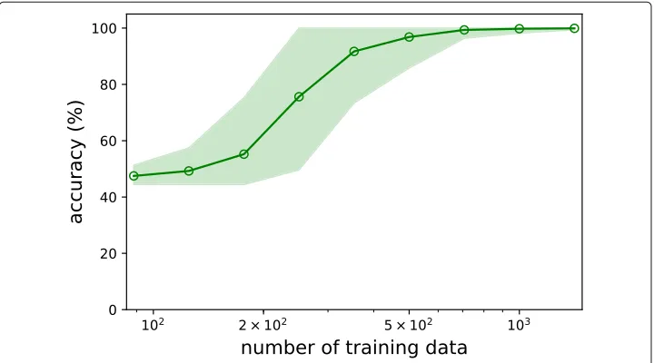
Reconstruction accuracy with data size
Fig. 6Accuracy of reconstruction in BA networks under different number of connections of each node
to a high deviation, which means that our method can either produce results with high accuracy or fail.
Conclusion
In this work we introduced GGN, a model-free, purely data-driven method that can simultaneously reconstruct network topology and perform dynamic prediction from time
series data of node state. Without any prior knowledge of the network structure, it is able to complete both tasks with high accuracy.
In a series of experiments, we demonstrated that GGN is able to be applied to a vari-ety of dynamical systems, including continuous, discrete, and even binary ones. And we found that in most cases, GGN can reconstruct the network better from non-chaotic data. In order to further explore GGN’s properties and to better know its upper limit, we con-ducted experiments under different network topology and different data volumes. The results show that the network reconstruction ability of our model is strongly correlated with the complexity of dynamics and the Clustering Coefficient of the network. It is also demonstrated that increasing the data size can significantly improve GGN’s net recon-struction performance, while a small data size can result in large deviation and unstable performance.
However, we are well aware that the current work has some limitations. It now focuses only on static graph and Markovian dynamics. Besides, as the limitation of our com-putation power, the maximum network size we can process is limited up to 100 nodes. Several possible approaches may help us to conquer these problems. First, if we can parameterize the network generator in a dynamical way, that is, to allow the generator parameters change along time, we can break through the limitations of static graphs. Second, if we replace the MLP network with RNN in the framework, learning of non-Markovian dynamics is possible. Third, to improve the scalability of our framework, node by node reconstruction of network can be adopted to save the space complexity. Another good way to improve the size limitation is to use graph convolution network (GCN) to model dynamics learner. GCN has been proved to be very useful in a large variety of field although it can not simulate some complex nonlinear process quite well from the experi-mental. In future works, we will further enhance the capacity of our model so as to break through these limitations.
Acknowledgements
We thank professor Wenxu Wang and Qinghua Chen from School of Systems Science, Beijing Normal University for discussion and their generous help.
Authors’ contributions
JZ conceived and designed the study. ZZ, YZ, SW, JL, RT and RX performed the experiments. ZZ, YZ, SW, JL, RT and RX wrote the paper. JZ reviewed and edited the manuscript. All authors read and approved the manuscript.
Funding
The research is supported by the National Natural Science Foundation of China (NSFC) under the grant numbers 61673070.
Availability of data and material
The datasets generated and/or analysed during the current study are available in https://github.com/bnusss/GGN.
Competing interests
The authors declare that they have no competing interests.
Author details
1School of Systems Science, Beijing Normal University, 100875 Beijing, People’s Republic of China.2ColorfulClouds Pacific
Technology Co., Ltd., No.04, Building C, 768 Creative Industrial Park, Compound 5A, Xueyuan Road, Haidian District, 100083 Beijing, People’s Republic of China.3School of Physics, Nanjing University, 210093 Nanjing, People’s Republic of
China.4Swarma Campus (Beijing) Technology Co., Ltd, 100083 Beijing, People’s Republic of China.
Received: 1 March 2019 Accepted: 23 August 2019
References
Albert R, Barabási A-L (2002) Statistical mechanics of complex networks. Rev Modern Phys 74(1):47
Battaglia P, Pascanu R, Lai M, Jimenez Rezende D, kavukcuoglu k (2016) Interaction networks for learning about objects, relations and physics. In: Lee DD, Sugiyama M, Luxburg UV, Guyon I, Garnett R (eds). Advances in Neural Information Processing Systems 29. Curran Associates, Inc. pp 4502–4510. http://papers.nips.cc/paper/6418-interaction-networks-for-learning-about-objects-relations-and-physics.pdf
Battaglia PW, Hamrick JB, Bapst V, Sanchez-Gonzalez A, Zambaldi V, Malinowski M, Tacchetti A, Raposo D, Santoro A, Faulkner R, et al (2018) Relational inductive biases, deep learning, and graph networks. arXiv preprint arXiv:1806.01261 Boccaletti S, Latora V, Moreno Y, Chavez M, Hwang D-U (2006) Complex networks: Structure and dynamics. Phys Rep
424(4-5):175–308
Boers N, Goswami B, Rheinwalt A, Bookhagen B, Hoskins B, Kurths J (2019) Complex networks reveal global pattern of extreme-rainfall teleconnections. Nature 566(7744):373–377
Bojchevski A, Shchur O, Zügner D, Günnemann S (2018) Netgan: Generating graphs via random walks. arXiv preprint arXiv:1803.00816
Brovelli A, Ding M, Ledberg A, Chen Y, Nakamura R, Bressler SL (2004) Beta oscillations in a large-scale sensorimotor cortical network: directional influences revealed by granger causality. Proc Nat Acad Sci 101(26):9849–9854 Casadiego J, Nitzan M, Hallerberg S, Timme M (2017) Model-free inference of direct network interactions from nonlinear
collective dynamics. Nat Commun 8(1):2192
De Cao N, Kipf T (2018) MolGAN: An implicit generative model for small molecular graphs. arXiv preprint arXiv:1805.11973 Eguiluz VM, Chialvo DR, Cecchi GA, Baliki M, Apkarian AV (2005) Scale-free brain functional networks. Phys Rev Lett
94(1):018102
Feizi S, Marbach D, Médard M, Kellis M (2013) Network deconvolution as a general method to distinguish direct dependencies in networks. Nat Biotechnol 31(8):726
Feurer M, Klein A, Eggensperger K, Springenberg J, Blum M, Hutter F (2015) Efficient and robust automated machine learning. In: Cortes C, Lawrence ND, Lee DD, Sugiyama M, Garnett R (eds). Advances in Neural Information Processing Systems 28. Curran Associates, Inc. pp 2962–2970. http://papers.nips.cc/paper/4824-imagenet-classification-with-deep-convolutional-neural-networks.pdf
Gardner TS, Di Bernardo D, Lorenz D, Collins JJ (2003) Inferring genetic networks and identifying compound mode of action via expression profiling. Science 301(5629):102–105
Guttenberg N, Virgo N, Witkowski O, Aoki H, Kanai R (2016) Permutation-equivariant neural networks applied to dynamics prediction. arXiv: Computer Vision and Pattern Recognition
He K, Zhang X, Ren S, Sun J (2015) Deep residual learning for image recognition. arXiv preprint arXiv:1512.03385 Hinton G, Deng L, Yu D, Dahl GE, Mohamed A-R, Jaitly N, Senior A, Vanhoucke V, Nguyen P, Sainath TN, Kingsbury B (2012)
Deep Neural Networks for Acoustic Modeling in Speech Recognition. IEEE Signal Process Mag 29(6):82–97 Jang E, Gu S, Poole B (2016) Categorical reparameterization with gumbel-softmax. arXiv preprint arXiv:1611.01144 Jain A, Zamir AR, Savarese S, Saxena A (2016) Structural-rnn: Deep learning on spatio-temporal graphs. In: Proceedings of
the IEEE Conference on Computer Vision and Pattern Recognition. pp 5308–5317
Kaneko K (1989) Pattern dynamics in spatiotemporal chaos: Pattern selection, diffusion of defect and pattern competition intermettency. Physica D: Nonlinear Phenomena 34(1-2):1–41
Kaneko, K (1992) Overview of coupled map lattices. Chaos: An Interdiscip J Nonlinear Sci 2(3):279–282
Kauffman SA (1969) Metabolic stability and epigenesis in randomly constructed genetic nets. J Theor Biol 22(3):437–467 Kipf TN, Welling M (2016) Semi-supervised classification with graph convolutional networks. arXiv preprint
arXiv:1609.02907
Kipf T, Fetaya E, Wang K-C, Welling M, Zemel R (2018) Neural relational inference for interacting systems. arXiv preprint arXiv:1802.04687
Krizhevsky A, Sutskever I, Hinton GE (2012) Imagenet classification with deep convolutional neural networks. In: Pereira F, Burges CJC, Bottou L, Weinberger KQ (eds). Advances in Neural Information Processing Systems 25. Curran Associates, Inc. pp 1097–1105. http://papers.nips.cc/paper/4824-imagenet-classification-with-deep-convolutional-neural-networks.pdf
Kuramoto Y (1975) Self-entrainment of a population of coupled non-linear oscillators. In: Araki H (ed). International Symposium on Mathematical Problems in Theoretical Physics. Springer, Berlin. pp 420–422
Li J, Wang W-X, Lai Y-C, Grebogi C (2015) Reconstructing complex networks with binary-state dynamics. arXiv preprint arXiv:1511.06852
Li Y, Yu R, Shahabi C, Liu Y (2017) Diffusion convolutional recurrent neural network: Data-driven traffic forecasting. arXiv preprint arXiv:1707.01926
Li Y, Vinyals O, Dyer C, Pascanu R, Battaglia P (2018) Learning deep generative models of graphs. arXiv preprint arXiv:1803.03324
Nadarajah S, Kotz S (2004) The beta gumbel distribution. Math Prob Eng 2004(4):323–332 Newman ME (2003) The structure and function of complex networks. SIAM review 45(2):167–256 Park H-J, Friston K (2013) Structural and functional brain networks: from connections to cognition. Science
342(6158):1238411
Quanming Y, Mengshuo W, Hugo JE, Isabelle G, Yi-Qi H, Yu-Feng L, Wei-Wei T, Qiang Y, Yang Y (2018) Taking human out of learning applications: A survey on automated machine learning. arXiv preprint arXiv:1810.13306
Quinn CJ, Coleman TP, Kiyavash N, Hatsopoulos NG (2011) Estimating the directed information to infer causal relationships in ensemble neural spike train recordings. J Comput Neurosci 30(1):17–44
Restrepo JG, Ott E, Hunt BR (2005) Onset of synchronization in large networks of coupled oscillators. Phys Rev E 71(3):036151
Shen Z, Wang W-X, Fan Y, Di Z, Lai Y-C (2014) Reconstructing propagation networks with natural diversity and identifying hidden sources. Nat Commun 5:4323
Strogatz SH (2001) Exploring complex networks. Nature 410(6825):268
Stuart JM, Segal E, Koller D, Kim SK (2003) A gene-coexpression network for global discovery of conserved genetic modules. Science 302(5643):249–255
Timme M (2007) Revealing network connectivity from response dynamics. Phys Rev Lett 98(22):224101 Veliˇckovi´c P, Cucurull G, Casanova A, Romero A, Lio P, Bengio Y (2017) Graph attention networks. arXiv preprint
Watters N, Zoran D, Weber T, Battaglia P, Pascanu R, Tacchetti A (2017) Visual interaction networks: Learning a physics simulator from video. In: Guyon I, Luxburg UV, Bengio S, Wallach H, Fergus R, Vishwanathan S, Garnett R (eds). Advances in Neural Information Processing Systems 30. Curran Associates, Inc. pp 4539–4547.http://papers.nips.cc/ paper/7040-visual-interaction-networks-learning-a-physics-simulator-from-video.pdf
Wang W-X, Yang R, Lai Y-C, Kovanis V, Grebogi C (2011) Predicting catastrophes in nonlinear dynamical systems by compressive sensing. Phys Rev Lett 106(15):154101
Wang W-X, Lai Y-C, Grebogi C, Ye J (2011) Network reconstruction based on evolutionary-game data via compressive sensing. Phys Rev X 1(2):021021
Wang W-X, Yang R, Lai Y-C, Kovanis V, Harrison MAF (2011) Time-series–based prediction of complex oscillator networks via compressive sensing. EPL (Europhys Lett) 94(4):48006
Watts DJ, Strogatz SH (1998) Collective dynamics of ’small-world’networks. Nature 393(6684):440
Yan S, Xiong Y, Lin D (2018) Spatial temporal graph convolutional networks for skeleton-based action recognition. https://aaai.org/ocs/index.php/AAAI/AAAI18/paper/view/17135
You J, Ying R, Ren X, Hamilton WL, Leskovec J (2018) GraphRNN: a deep generative model for graphs. arXiv preprint arXiv:1802.08773
Yu B, Yin H, Zhu Z (2017) Spatio-temporal graph convolutional networks: A deep learning framework for traffic forecasting. arXiv preprint arXiv:1709.04875
Zhang J, Shi X, Xie J, Ma H, King I, Yeung D-Y (2018) Gaan: Gated attention networks for learning on large and spatiotemporal graphs. arXiv preprint arXiv:1803.07294
Zonghan W, Shirui P, Fengwen C, Guodong L, Chengqi Z, Philip SY (2018) A comprehensive survey on graph neural networks. arXiv preprint arXiv:1901.00596
Publisher’s Note