L410 Simulation - Initial Conditions, Flight Dynamics

(1)

L410 Simulation - Initial Conditions, Flight

Dynamics

Rudolf Volner, LETS FLY s.r.o.,

International Airport Ostrava, Mošnov 403, Czech republic,

Ľubomír Volner

Transport Research Institute in Žilina, Slovak republic

Abstract - This article describes one of the possibilities of simulating the flight parameters of the aircraft L 410 UVP - E20 with the help of Matlab/Simulink. The article focuses on the definition of basic algorithms and the possibility of applying these algorithms using software such as Matlab/Simulink.

Keywords—simulation, aircraft, L410, model

I. INTRODUCTION

Flight L-410 Turbolet is a Czech transport and transport airplane designed for regional transport. It is a high-rise, self-supporting monoplane. The fuselage consists of all-metal half-shell, the wing is two-armed, equipped with double-wing flaps and spoilers. The propulsion unit consists of two Walter M 601 turboprop engines and an Avia V508 or V 510 propeller - a fixed-speed propeller with the ability to fire and reverse. The electrical system is powered by a direct voltage of 28V. The aircraft is equipped with a main and backup hydraulic system. The chassis is hydraulically retractable. The machine is capable of landing in small and untouched aerodromes and capable of operating under extreme conditions from +50 ° C to -40 ° C, is certified for IFR, accurate ILS CAT 1 approach. Over 1 100 pieces were produced, the main the buyer of airplanes was Soviet Aeroflot, but were further re-sold to countries in Asia, Africa and South America [12].

Another variant was the L-410UVP (STOL), which has an extended fuselage, an enlarged wing span and stabilizer uplift was adjusted to + 7 °. An automatic bank control (ABC) has been added to the automatic battle system. This is a wing at the end of the wing, which opens automatically when a single engine fails, but only at a speed of 205km/hour. The wing was equipped with interceptors. Equipment and brakes have been improved. First, the M601B engines with the same performance were installed, but at higher temperatures it was more efficient, but the M601D and the V508D propellers were later installed. The number of seats is 15. The take-off is approximately 456 m

[12]

.

The most common variant is the L-410UVP-E with increased maximum take-off mass, stronger

Walter M601E engines, five-propelled V510

propellers. At the end of the wings, external (sometimes mistakenly called additional) tanks can be mounted. The prototype took off in 1984 and started production in 1985. There are other UVP-E submarines: UVP-E9 and UVP-E20, which differ in detail due to the periodic requirements for complying with JAR 25 and, respectively, FAR-23. The latest version of the Turbolet is the L-420 with the M601F, which has been certified by the US FAA. The L-410 versions M to E (including E9 and E20) have a type certificate issued by EASA [12].

II. Defining aircraft geometry (General Aircraft Geometry, model L-410)

Potential power requirements for this aircraft:

 Travel speed,

 Acceptable climb speed,

 Acceptable lowest critical speed.

(2)

reliable. It is almost always necessary to make certain simplifications, ie. establish models of flow fields, or the aerodynamic characteristics obtained experimental way.

The starting point for the model is the similarity analysis parameters and circumstances on which the aerodynamic force depends. If the aerodynamic forces acting on the aircraft at regime forces are generally dependent on:

 The parameters of the body - size, shape,

configuration of the body to high pressure (determined by the angle of attack α),

 Current parameters - speed V, specific gravity

ρ (characterized by flight altitude h), viscosity

μ, compressibility (speed of sound a).

Flight performance means that part of the flight mechanics, which deals with the center of gravity in relation to a flight mode or maneuver. Addresses the speed, time, path length and seek their extremes (minimum and maximum speed, the maximum rate of climb, maximum flight time - perseverance, the maximum flight path - down and more). Performances and represent the kinematics flight modes and maneuvers unrelated to the pilot.

In principle, flight performance can be divided into performances of airplane performance and the performance of transient modes. Steady flight modes are modes with constant speed and straight-forward (horizontal flight, climb, glide) and curvilinear (cornering). Unsteady modes are flights with variable speed, following direct or curvilinear paths. Because the procedures related to the center of gravity, do not stand in equilibrium equations of motion and torque characteristics.

Flight characteristics on monitoring the movement of aircraft in terms of piloting, respectively, in terms of managing the aircraft. It assesses the stability of the flight regime, requirements for regime change in power management and more.

IV.Simulation initial conditions and Dynamics simulations of flight

flight procedures.

(3)

Fig. 4. The initial conditions [13]- [17]

Fig. 5 Dynamics simulations of flight [13]- [17]

V. Determination of aerodynamic vehicle characteristics

The geometric layout of the aircraft determines its aerodynamic properties, so its performance and handling characteristics. After selecting the geometric configuration, aerodynamic properties can be obtained by:

 Analytical prediction,

 Wind tunnel testing from the model or full

prototype size,

 flight tests.

While wind tunnel and flight test tests provide good results, they are expensive and time-consuming because they have to be performed on real hardware. Analytical prediction is a faster and less costly way of estimating aerodynamic characteristics in the early design phases.

In this example, we will use DIGITAL DATCOM, a popular software program, for analytic prediction. This software is publicly available.

(4)

technical computing.

In the model we have to check whether the vehicle is by its nature stable. For this, we can use Fig. 2 to verify that the rising moment described by the

respective coefficient Cm provides the return torque for

the aircraft. The return torque returns the plane of the aircraft to zero.

In configuration 1 – fig. 2, Cm is negative for some

rise angles less than zero. This means that this configuration will not provide a return torque at those negative startup angles and will not provide the flight characteristics that are desirable. Configuration 2 addresses this problem by shifting the center of gravity backwards. The displacement of the center of gravity

produces Cm, which provides a return torque for all

negative offset angles.

Fig. 2 Digital Data Coefficients of the Climate Moment Visual Analysis

VI.Design of control flight laws

After creating the model in Simulink, we design a longitudinal controller that controls the position of the elevator for height control. Fig. 9 shows the external height control loop (C1 compensator yellow) and the internal loop for controlling the climb angle (C2 compensator blue). Fig. 10 shows the corresponding configuration of the Simulink controller.

The controller can be set directly in Simulink using various tools and techniques.

Using the Simulink Control Design interface, we have introduced a control problem by specifying:

 Two Controller Blocks,

 Closed circuit input or altitude command,

 Output signals in closed loop or sensor height,

 Steady or trimmed.

Using this information, Simulink Control Design

software automatically calculates linear

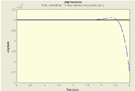
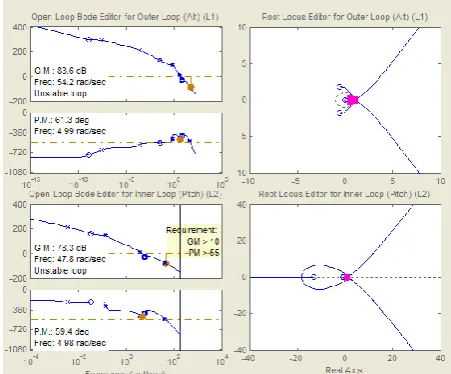
approximations of the model and identifies feedback loops to be used in the design. To design the controllers for the inner and outer loops, we use root locus and point plots for the open loops and a step response plot for the closed-loop response – Fig. 11.

(5)

Fig. 11 Map design before debugging the controller

Subsequently, it is possible to interactively adjust the compensators for the inner and outer loops using these maps.

To make the loop design more systematic, a sequential loop closure is used. This technique allows us to gradually take into account the dynamics of other loops during the design process. Simulink Control Design, sets the internal loop to have another loop hole at the output of the outer loop controller - C1 in Fig. 12. This approach separates the inner loop from the outer loop and simplifies the construction of the internal loop controller. After designing the inner loop, we suggest an outer loop controller. Fig. 13 shows the resulting perfect embodiment of the compensator.

Fig. 12 Block diagram of an internal loop, isolated by configuration of the supplementary opening of the loop

Fig. 13 Map design in trim state after tuning the controller

The controller can be tuned in different ways, for example:

 We can use the graphical approach and interact

with the gain of the controller, poles, zeros until we get a satisfactory response – Fig. 13,

 Simulink® Design Optimization ™ software

can be used for automatic tuning.

After specifying the frequency domain

requirement, such as gain and margin phase and time zone requirements, Simulink automatically tunes the controller parameters to meet these requirements. Once the acceptable design of the controller has been developed, the control blocks in the Simulink are automatically updated.

Fig. 15 shows the simulation results of a closed loop of the nonlinear Simulink model for the desired height increase from 2000 m to 2050 m.

Fig. 14 The final check is to start the nonlinear simulation with the proposed controller, and check whether the height (purple) follows the height requirement (yellow) in a stable

and acceptable way

(6)

estimate its performance and manageability much longer than any hardware is built, which reduces design costs and eliminates errors.

ACKNOWLEDGEMENTS

The article was prepared within the project

TA04031376 „Research/development training

methodology aerospace specialists L410 UVP - E20“. This project is supported by Technology Agency Czech Republic.

REFERENCES

[1] Volner, R. a kol. Flight Planning

Management, Akademické nakladatelství CERM s.r.o.

Brno, 2007, ISBN 978-80-7204-496-2, 630 str., [in Czech]

[2] Volner, R. Modelovanie a simulácia, Verbum

KU Ružomberok, 2014, ISBN 978-80-561-0165-0, 209 str., [in Slovak]

[3] Vavroš, P., Volner, R. “Aplikácia

modelovania a simulácie vo výcviku leteckých

špecialistov”, Perner´s Contacts - Elektronický

odborný časopis, pp. 186 - 195, 1/2015, ročník X, duben 2015, Univerzita Pardubice, ISSN 1801 – 674X, str. 195, [in Slovak]

[4] The USAF Stability and Control Digital Datcom, AFFDL-TR-79-3032, 1979

Corporation Team Aircraft Design Competition, 1991-1992.

[9] Turvesky, A., Gage, S., and Buhr, C.,

“Accelerating Flight Vehicle Design”, MATLAB® Digest, January 2007.

[10] Turvesky, A., Gage, S., and Buhr, C., “Model-based Design of a New Lightweight Aircraft”, AIAA paper 2007-6371, AIAA Modeling and Simulation Technologies Conference and Exhibit, Hilton Head, South Carolina, Aug. 20-23, 2007.

[11]https://aerofred.com/categories.php?cat_id= 4&sessionid=87217bs5f8cr8s05rnmpetffo7&page=32 8

[12]https://cs.wikipedia.org/wiki/Let_L410_Tur bolet

[13] Aircraft Industries, a.s., Aircraft flight

manual for the L 410 UVP-E, Kunovice, 2005, book 1

manual for the L 410 UVP-E, Kunovice, 2005, book 2

manual for the L 410 UVP-E20 with H80-200 Engines and AV-725 Propellers, Kunovice, 2013

[16] Aircraft Industries, a.s., Aircraft training

book L 410, Kunovice, 2012, book 1

[17] Aircraft Industries, a.s., Aircraft training