Cyclic Convolution Algorithm Formulations Using Polynomial Transform Theory

(1)

Cyclic Convolution Algorithm Formulations

Using Polynomial Transform Theory

Abraham H. Diaz-Perez

Popular University of the Cesar/ Electronic Department, Sabanas Campus, Valledupar-Cesar, Colombia Email: [email protected]

Domingo Rodriguez

University of Puerto Rico/ Electrical and Computer Engineering Department, Mayagüez PR. 00681-9042 E-mail: [email protected]

Abstract— This work presents a mathematical framework for the development of efficient algorithms for cyclic convolution computations. The framework is based on the Chinese Reminder Theorem (CRT) and the Winograd’s Minimal Multiplicative Complexity Theorem, obtaining a set of formulations that simplify cyclic convolution (CC) computations. In particularly, this work focuses on the arithmetic complexity of a matrix-vector product when this product represents a CC computational operation or it represents a polynomial multiplication modulo the polynomial zN-1, where N represents the maximum length of each polynomial factor and it is set to be a power of 2. The proposed algorithms are compared against existing algorithms developed making use of the CRT and it is shown that these proposed algorithms exhibit an advantage in computational efficiency. They are also compared against other algorithms that make use of the Fast Fourier Transform (FFT) to perform indirect CC operations, thus, demonstrating some of the advantages of the proposed development framework.

Index Terms—Cyclic Convolution, Fast Fourier Transform, Circulant Matrix, Winograd’s Theorem, Chinese Remainder Theorem.

I. INTRODUCTION

In digital signal processing, the design of fast and computationally efficient algorithms has been a major focus of research activity. The objective, in most cases, is the design of algorithms and their respective implementation in a manner that perform the required computations in the least amount of time. In order to achieve this goal, parallel processing has also received a lot attention in the research community [1].

This paper summarizes the main properties of the CC, or the polynomial multiplication modulo the polynomial

zN-1, when they are represented by a vector-matrix multiplication operation using a circulant matrix [2].

Direct computation of a matrix-vector product takes 2

N complex multiplications; however, by exploiting the special structure of a circulant matrix, the computational effort could be substantially decreased for large matrices. One approach is to use the fast Fourier transform (FFT), which makes possible to compute a matrix-vector product in (N)log₂(N) complex multiplications for a matrix of order N. In this work algorithms are developed by means of a decimation in time approach, and the use of the roots of the unity (factoring the polynomial zN-1in the complex field). They require only N multiplications, with some advantages over FFT such as memory use and addressing techniques.

In the present work the CRT and the Winograd’s theorem are used for the formulation of new and computationally efficient algorithms for matrix-vector products when they represent cyclic convolution operations. The mappings of the resulting operations onto signal flow diagrams that imply parallel computation are also remarked.

This document is organized as follows. First, mathematical foundations needed for the study of algorithms to compute the discrete convolution are summarized. Second, an identification is established between products of polynomials and the convolution operation. Third, the algorithm development for the basic problem of the multiplication of a circulant matrix by a vector, using the conceptual framework developed in the two previous sections, is explained. The section also presents several signal flow diagrams that may be implemented in diverse architectures by means of very large scale integration (VLSI) or very high speed integrated circuits hardware description language (VHDL) [3]-[8]. Conclusions, contributions, and future development of the present work are then summarized.

(2)

II. THEORETICAL FRAMEWORK

A. Discrete Linear Convolution

A block diagram representing a basic discrete system is depicted in Figure 1 below. A discrete system is defined here as an entity which acts, transforms, or operates on a input signal, termed the input signal in order to produce another signal, termed the output signal [9]. An important class of discrete systems is linear and shift-invariant systems known as discrete filters. A discrete filter is uniquely described by its impulse response signal, denoted by [ ], h n nZ , where Z is the set of integers. A discrete filter’s impulse response is obtained as a resulting output signal when the input to the filter is a delta function G[ ], n nZ, with [ ] 1G n for

0

n andG[ ]n 0for nz0. Consider an arbitrary input signal x n[ ], nZ, to a discrete filter with an associated impulse response signal equal to [ ], h n nZ. The output signal, say y n[ ], nZ , of the discrete filter is given by the following general expression.

[ ] m [ ] [ ] m [ ] [ ],

m m

y n fx m h n m fh m x n m n Z

f f

¦ ¦

This operation is commonly known as the linear convolution sum operation of the input signal

[ ],

x n nZ with the impulse response signal

[ ],

h n nZand it is commutative operation.

Figure 1

The set of all discrete complex signals of the type

[ ],

x n nZbecomes a linear space denoted by l Z( ). A subspace of this linear space, denoted by l2( )Z , is the set of all discrete signals with finite energy. A discrete signal, say x n[ ], nZ, is said to have finite energy if the condition n [ ] [ ]* ,

n

x n x n x x

f f

f

¦ is satisfied. The

symbol “*” in the expression above denotes complex conjugation. The expression x y, is termed an inner product of x and y, with, both, x y, l2( )Z . The norm or length of a finite energy discrete signal xl2( )Z is denoted by _x _{x x}_, 12_.

A very important subset of the linear space l2( )Z is the set of finite discrete complex signals of length or order, say, N. This subset is denoted by l2(Z_N)and it is itself a linear space of vector space of dimension N. The set Z_N {0,1, 2,",N1}is called the standard finite indexing set. Each element of the space l2(Z_N)is of the form x Z: _N oC, where Cis the set of complex numbers and the valuationx n[ ]is a complex number. A signalxis represented in this work as a column vector.

An inner product of two finite sequences, say x and y, can be defined in the linear space or vector space

2

( )

l Z through the expression

1 * 0

, [ ] [ ] ,

N

n

x y ¦ x n y n z y x , with x y, Cbeing a complex number. The length or norm of a finite signal

2

( N)

xl Z is then _x _{x x}_, 12_{. An identification is made} in this work between the linear space or vector space

2

( )

l Z , the vectors belonging to the complex Euclidean space CN, and the finite dimensional polynomial algebraC x[ ] /xN1, the ring of polynomials C x[ ]

modulo the monic polynomial xN1 . The inner product

2

, , , ( _N)

x y x yl Z can be then identified with the standard Euclidean metric in CN.

It is important to point out that the linear space l2( )Z can be turned into a finite dimensional linear algebra by introducing a vector multiplication operation [10]. There are many operations that can be used as a multiplication operation in l2( )Z . One of the most useful multiplication operations utilized is the cyclic convolution operation modulo N. In the next section this cyclic convolution operation is introduced along with some of its most important properties.

B. Periodic or Cyclic Convolution

Let x h, l2(Z_N)be two arbitrary sequences, each of length N. The periodic or cyclic convolution modulo N

of these two signals is denoted by the expression x_Nh

and it is a new signal, say y, also of length N, defined by the following expression for any nZ_N:

1 0 1 0

[ ] [ ] [ ] [ ]

or

[ ] [ ] [ ] [ ]

N

N _N

m N

N _N

m

y n x h n x m h n m

y n h x n h m x n m

¦

Here, the notation N

p , implies the remainder p

after being divided by N.

The focus of this work is to develop fast and efficient algorithms for the computation of the circular or cyclic convolution operation, reaching the minimal number of multiplications according to the Winograd’s theorem. Normally, two approaches are utilized to compute the cyclic convolution operation, namely, the direct approach and the transform approach. The direct approach evaluates the equation for the cyclic convolution of two

N- point signals for each value nZ_N resulting in a system of equations. The transform approach establishes a discrete Fourier transform (DFT) isomorphism between the cyclic convolution operation two signals in the object domain and the point-by-point multiplication operation or Hadamard product of each of the transformed signals. Discrete System

x[n]

(3)

C. Matrix Representation of the Cyclic Convolution

This section describes a cyclic convolution operator as a linear shift invariant (LSI) operator acting on the finite dimensional linear space

l Z

2

(

N

)

. In addition, the cyclic

convolution operator is also described as a cyclic finite impulse response (FIR) system. Combining these two attributes allows for a deeper study of the properties of the cyclic convolution operator. A formal discussion follows, arriving at a matrix representation of a cyclic convolution operation [11].

Since each N-dimensional LSI-FIR system

2 2

: (

(

)

h N N

T l Z

o

l Z

describes a linear mapping on

the space

L Z

_N , each

T

_h is uniquely determined by its action on a set of basis vectors (signals) spanning

N

Z

l

2 . If the standard basis set

^

G

_{^ `}_j

:

j

Z

_N

`

is chosen

as reference, then each signal

T

_h

G

_{^ `}_j

L Z

_N

can be uniquely expressed as a linear combination of the basis set:

^ `

> @

^ `j Z

j k h

N

k

j

h

T

G

_¦

G

,

}

{ ,

where the set of scalars

^

h

> @

j

,

k

:

j

Z

_N

`

,

k

Z

_N

actually represents the vector coordinates of the given signal

T

_h

^ `

G

_{^ `}_k

,

k

Z

_N , with respect to the standard basis set. The signal

T

_h

^ `

G

_{^ `}_k can be written as follows:

^ `

¦

^ `

> @

^ ` ZN

j

j k h k

h

T

j

T

G

,

where

^ `

> @

^ `

> @

N

m

h k N k

m Z

T

G

j

h m S

G

j

¦

^ `

> @

^ `

> @

N

h k k m

m Z

T

G

j

h m

G

j

¦

h

> @ >

m

j

k

m

@ >

h

j

k

@

S

_Nk

^ `

h

> @

j

Z m N

¦

G

Thus, the following formulation may be obtained

^ `

> @

^ `

>

@

^ `j Z

j j Z

j k h

N N

k

j

h

k

j

h

T

G

_¦

G

_¦

G

,

^ `

> @

^ `

_{^ `}

^ `

¦

S

_Nk

h

j S

T

h

S

h

j Z

N j

S h N

k

N

N k

G

It is important to point out that the expression

S

_Nm

^ `

G

_{^ `}_k represents the action of the cyclic shift operation over an the

k

-th element of the ordered standard basis set. This operator action is formally defined as follows:

^ `

_^

_`

2 2

:

(

)

(

)

N

m

N N N

m N

k k k m

S

l Z

S

G

o

6

The notation

N denotes modulo

N

arithmetic, which we will omit most of the time for better readability.

Next, the matrix HN formally is defined as follows:

> @

>

@

>

@

H

_N

h j k

h j

k

j k ZN j k ZN

,

, ,

The matrix HN , thus, have the following form

> @

>

@

>

@

> @

>

@

> @

>

@ >

@

> @

»

¼

º

«

¬

ª

0

3

2

1

3

0

1

2

1

0

1

2

1

0 h

N

h

N

h

N

h

N

h

N

h

N

h

H

N

"

#

"

Notice that the columns of HN are formed by cyclic shifted versions of the coordinate vector representation of the signal h with respect to the standard basis set; that is, the matrix HN can be written as the following ordered action of the cyclic shift operator:

^ `

>

I

h

S

h

S

h

S

h

@

H

N N N N NN

1 2

,

!

To describe in more details how the matrix HN, representing the system Th, is obtained, the action of the operator over an element of the standard basis is formulated as follows:

^ `

h

> @

j

k

S

^ `

h

> @

j

k

C

T

N

Z j

j N k

h

¦

,

G

^ `k

> @

0 ,

^ `0

> @

1 ,

^ `1

>

1 ,

@

^N1`

h

k

h

k

h

N

k

T

G

!

G

Evaluating this expression at different values of

k

Z

_N results in the following set of identities:

^ `

0

> @

0 ,

0

^ `0

>

1 ,

0 @

^N1`

h

N

T

G

"

G

^ `

1

> @

0 ,

1

^ `0

>

1 ,

1 @

^N1`

h

N

T

G

"

G

^ `

^

N1

`

>

0 ,

1 @

^ `0

>

1 ,

1 @

^N1`

h

N

h

N

T

G

"

G

Rewriting these identities in array form results in:

^ `

^

`

> @

>

@

> @

>

@

>

@

>

@

^ `

»

¼

º

«

¬

ª

»

¼

º

«

¬

ª

»

¼

º

«

¬

ª

1

1 0

1 1 0

1 ,

1

1 ,

0

1 ,

1

1 ,

0

0 ,

1

0 ,

0

N N

h h h

N

h

N

h

N

h

N

h

T

G

#

Thus, given a system Th, and a signal

f

L Z

_N , a response

g

T f

_h

^ `

is obtained as follows:

^ `

> @

^ ` N

h h j

k Z

g

T

f

T

f k

G

½

¦

®

¾

¯

¿

(4)

Taking advantage of the linearity of

T

_h results in:

^ `

> @

^ `

> @

^ `

N N

h h k j

k Z j Z

g

T

f

f k T

G

g j

G

¦

Thus,

^ `

> @

_{^ `}

,

2

N

h j N

j Z

g

T

f

g j

G

f

l

Z

¦

, or

^ `

> @ > @

^ `j Z

j k Z

h

N N

k

j

h

k

f

T

g

_{¦ ¦}

G

¸

¹

· ¨

¨

©

§

,

, where

> @

m

T

^ `

f

> @ > @

k

h

j

k

^ `

> @

m

g

_j

Z j k Z h

N N

G

¸

¹

· ¨

¨

©

§

¦ ¦

,

> @ >

@

¦

N

Z K

N

Z

m

k

m

h

k

f

m

g

[

]

,

This last expression in coordinates notation with respect to the standard basis results in the following expression:

> @

>

@

> @ > @

> @ >

@

»

¼

º

«

¬

ª

»

¼

º

«

¬

ª

_¦

¦

1 0

1 0 1 0

,

1 ,

,

1 ,

0

1

0

N

k N

k

N

h

k

f

k

j

h

k

f

k

h

k

f

k

h

k

f

N

g

j

g

#

Extracting the f from the above, results in the following matrix-vector representation

> @

>

@

> @

>

@

> @

>

@

>

@

>

@

>

@

>

@

0 0, 0

0,

1

1 1, 0

1,

1 , 0

,

1

1 1, 0

1,

1 g

h

N

g

h

N

f

g j

h j

h j N

g N

h N

N

ª

º

ª

º

«

»

«

»

«

»

«

»

«

»

«

»

«

»

«

»

«

»

«

»

«

»

«

»

«

»

«

»

«

»

«

»

¬

¼

¬

¼

"

#

%

#

"

#

"

Recalling that

h j k

>

,

@

h j

>

k

@

,

j k

,

Z

_N, produces the following expression for the matrix-vector formulation of the cyclic convolution operation:

> @

>

@

> @

>

@

>

@

> @

>

@

0

1

0

1

2

1

0

1 g

h

f

g

h

f

g j

h j

f j

g N

h N

h

f N

ª

º

ª

º ª

º

«

»

«

» «

»

«

»

«

» «

»

«

»

«

» «

»

«

»

«

» «

»

«

»

«

» «

»

«

»

«

» «

»

«

»

«

» «

»

«

»

«

» «

»

¬

¼

¬

¼ ¬

¼

"

#

%

#

"

#

"

Thus, the matrix-vector computation

g

H

_N

f

represents the cyclic convolution operation of the vectors

f

and

h

, or simply,

g

f

_N

h

T

_h

^ `

f

. Since the vector or signal

f

is an arbitrary vector, a general formulation for the matrix

H

_N is given, where commas are used to improve readability of the expressions:

^ `

^

^ `

`

>

h 0

,

h 1

,

h N1

@

N

T

H

G

!

G

^ `

>

T

h

T

h

T

h

@

H

N

N G0

,

G1

,

!

,

G 1

^ `

>

G

h

G

@

N N h

N h

N

I

T

S

T

S

T

H

1

,

!

The cyclic convolution operation can now be formulated at the vector space or linear space level as follows:

^ `

N

h

N

h

T

f

h

L

Z

f

g

,

^ `

> @

^ `

¸

¹

· ¨

©

§

¦

1

0

N

k

k h

h

f

T

f

k

T

g

G

^ `

> @

^ `

¿

¾

½

¯

®

¦

ZN

k

k h

h

f

T

f

k

T

G

^ `

¦

> @

^ `

^ ` ZN

k

k h

h

f

k

T

G

^ `

¦

> @

¦

>

@

^ `

¸

¹

· ¨

¨

©

§

N N

Z

k j Z

j

h

f

k

h

j

k

T

G

^ `

>

@ > @

^ `j Z

j k Z

h

N N

k

f

k

j

h

f

T

_{¦ ¦}

G

¸

¹

· ¨

¨

©

§

Evaluating

g

l

2

Z

_N at

j

Z

_N results in

> @

^ `

> @

¦ ¦

>

@ > @

^ `

> @

¸

¹

· ¨

¨

©

§

N N

Z j

j Z

k

h

f

j

h

j

k

f

k

j

T

j

g

G

> @

>

@ > @

N N

j Z k Z

g j

h j

k f k

G

§

· ¦

_¨

¦

_¸

©

¹

>

@ > @

[ ]

N

k Z

g j

h j

k f k

¦

.

(5)

Consider the Nequations for cyclic convolution:

1 1

0 0

[ ] N [ ]. [ _N] N [ ]. [ _N]

m m

y n ¦ h m x n m ¦ x m h n m ,

0,1, 2,

,

1 n

"

N

In matrix form these equations may be expressed as:

[0]

[

1 [1]

[0]

[1]

[0]

[2]

[1]

[

1]

[

1]

[

2]

[0]

[

1]

y

x

x N

x

h

y

x

h

y N

x N

x

h N

ª

º ª

ºª

º

«

» «

»«

»

«

» «

»«

»

«

» «

»«

»

«

» «

»«

»

¬

¼ ¬

¼¬

¼

"

#

%

#

"

Note: A matrix A is a Toeplitz-like matrix if the elements along the diagonals are the same. That is, if:

pq ij a

a forip jq

If the matrix A is of sizeNuN and each row is the preceding row circularly rotated right, then the matrixA is termed circulant [12]. The matrix representation of the CC is a circulant matrix.

D. The Discrete Fourier Transform (DFT)

Given a discrete signalxl2(Z_N), then the discrete Fourier transform (DFT) pair is established as follows:

¦

1

N

0 n

kn W ]. n [ x ] k [

X ļ

¦

1 N

0 k

nk W ]. k [ X N

1 ] n [ x

Here,Nis the number of samples in one period of

2₍ ₎

N

xl Z , and )

N 2 j exp(

W S .

A cyclic convolution property relates the resulting cyclic convolution signaly of two periodic discrete signals x y, l2(Z_N)by means of their DFT in the following manner:

1 N ,..., 1 , 0 k ] k [ X ] k [ H ] k [

Y

Here, Y[k],H[k] and X[k] are the DFT’s of y, h, andx, respectively. Thus, an alternative formulation of the CC is as follows:

1 N ... 2 , 1 , 0 n W ] k [ X ] k [ H N

1 ] n [ y

1 N

0 k

nk

¦

] k [

H and X[k] can be computed in parallel and then calculate the Nproducts H[k]X[k] kZN.

E. Polynomial Congruences.

An nth degree polynomial P[z] over some field F is formulated by the following expression:

0 n z a ] z [ P

n

0 i

i

i !

¦

,

where the fixed elements {a_i} are drawn from the field F, normally a Galois field GF(p)or an isomorphic subset of the complex numbers. Some of the elements can be zero but a_n cannot. If a_n is the unity, then the polynomial is termed a monic polynomial.

Thedegree ororder of the polynomial is denoted by

]] z [ P [

Deg . Assume two polynomials P[z] and Q[z]

meet this definition. If there exist a third polynomial

] z [

D such that P[z] Q[z]D[z], then D[z] is termed a divisor of P[z]and the division is denoted by

] z [ P ] z [

D .If P[z] can only be divided by polynomials of degree 0 (that is numbers) or polynomials of degree n, then P[z] is termed irreducible over the field F or

prime [5]. The structure of the monic polynomials

] z [

p_i is strongly dependent on the field F. The classic example is (z21) which is irreducible in the real numbers field, in the rational field, and the integer field; however, it has factors (zi) and (zi) in the complex field. The nature of field, then, plays an important role in the minimal algorithms for products of polynomials [13], as will be demonstrated in the next sections.

Associated with a N-point discrete signal or sequence [ ], _N

y n nZ , or simply [ ]y n , there exist an (N1)-th

degree polynomial in the indeterminate

z

: 1 1 1

0 ... )

(

N N z

y z y y z y

If a sequence y[n] is the convolution of two sequences h[n] and x[n], then a well-known property of z transform is expressed as follows:

] z [ X ] z [ H ] z [

Y

Where Y[z],H[z] and X[z] are the z transform of

] n [

y , h[n] and x[n] respectively. Thus, efficient methods for convolving sequences are also efficient methods for multiplying two polynomials, and vice versa. Consider the general polynomial congruence:

] z [ P ] z [ X ] z [ H ] z [

Y

where H[z] andX[z] are two polynomials defined over the same field as Y[z]. Given the inequality:

]) z [ X ( Deg ]) z [ H ( Deg ]) z [ P (

Deg ! ,

then this describes a discrete convolution operation. If all three polynomials have degree of N and P[z] is the polynomial (zN 1), then the cyclic convolution can be represented as a multiplication of polynomials modulo a monic polynomial through the expression:

) 1 (

) ( ) ( )

(z x z h z _zN

y

F. Winograd’s Minimal Complexity Theorem.

Let F be an arbitrary field and let { }[ ]F z represent the linear space of all polynomials in the indeterminate

z, with degree less than N. Let X z H z[ ], [ ] { }[ ] F z

two polynomials defined over the field F. Then, the operation:

] z [ P ] z [ X ] z [ H ] z [

Y

(6)

This last number N is the number of complex multiplications obtained by the application of the proposed algorithms demonstrated in the next section.

G. The Chinese Remainder Theorem (CRT).

Optimal algorithms for one dimensional cyclic convolution have been constructed by Winograd [6] by means of the CRT. Consider the expression for polynomial multiplication modulo a polynomial:

) (

) ( ) ( )

(z x z h z pz

y

With,

k

i i z p z p

1

) ( )

(

The polynomial product can be reduced to the following product of polynomial of smaller degree:

) (

) ( ) ( )

( i i _p _z

i

z h z x z

y , and the total product can be

reconstructed using the Chinese Remainder Theorem (CRT) [7] by:

¦

k i

z p i i z R z

y z

y

1

) (

) ( ) ( )

(

The polynomials R_i(z) are defined as:

j i z p

z p z

R

j i i

z

), ( mod 0

), ( mod 1 ) (

In [5] is demonstrated that the products y_i(z) are disjoint. It is also proved that if optimal algorithms for the products y_i(z) exist, then the algorithm together with the polynomial reductions modulo pi(z) and the CRT

reconstruction form an overall optimal algorithm for the computation of the cyclic convolution [8].

III. ALGORITHM DEVELOPMENT

This section shows the process to obtain recursive algorithms in order to perform the polynomial product of length N modulo the polynomial _p(_z) (_zN1)_when

N is a power of 2. In the development a matrix representation is used to formulate a matrix-vector product and take advantage of the structure of the circulant matrix and the roots of unity. In this manner a lower bound is obtained in the number of multiplications as established by the Winograd theorem.

Lety Xh, whereN 2, and N1 1 is the degree of the associated polynomials, the polynomial product module (z21) can be represented in matrix form as:

» ¼ º «

¬ ª

»

¼ º « ¬ ª » ¼ º « ¬ ª

0 1 1 0

1 1 0 0 1 0 0 1

1

0 _.

h x h x

h x h x h h x x

x x

y ₍₁₎

Straightforward computation is done by means of 4 multiplications and 2 sums. Winograd in [6], [7] shows that, for computing this matrix-vector product, the following algorithm can be used with only 2 multiplications and 6 sums:

: where , .

2 1

2 1 1 0 0 1

1 0

» ¼ º «

¬ ª

» ¼ º « ¬ ª » ¼ º « ¬ ª

m m

m m h h x x

x x y

) )( ( 2 1 ); )( ( 2 1

1 0 1 0 2 1 0 1 0

1 x x h h m x x h h

m ₍₂₎

In the reduction of the algorithm’s complexity in terms of multiplications, it is not necessary to take into consideration the multiplications by

2 1

,1 and 1. They

are elements of the field of constants or ground set G, which will be in the field of complex numbers [6], [7]. The following observation can be made: the constants employed in this algorithm are the roots of unit of the polynomial _zN 1

in this case z21 (1and1), and the value

2 1

is simply

N 1

. The relation between this

algorithm for performing cyclic convolution and the approach using the DFT is now evident, since the constants used in both algorithms are the same.

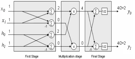
The following figure shows, through a numerical example, how the first algorithm can be mapped into a parallel hardware structure:

Figure 2. Flow diagram for cyclic convolution - N=2.

The Figure 2 above shows three stages in the algorithm for N 2. The first stage can be associated with the DFT. In fact, the values of the coefficients at the output of this stage are the same that those obtained by applying the DFT. The multiplication stage can be associated with the Hadamard multiplication product of the two transformed sequences, and the last stage can be related to the inverse transform. The number of stages of our algorithm is given by the order of the sequences. In this case, for N 21, the algorithm shows S₁ log₂(N) 1

multiplication stages by the field of constants or ground set G(the roots of the polynomial 2 1

z ), and

1 ) ( log₂

2 N

S multiplications stages by the roots of the polynomial z21. It is necessary only one stage to multiply the sequences and it is of sizeN, which is the limit established by the Winograd theorem. Now, increasing the order of the polynomials to the next power of two, which is N 22 4, the matrix representation is then:

, and

,

3 2 1 0

0 1 2 3

3 0 1 2

2 3 0 1

1 2 3 0

» » » » »

¼ º

« « « « «

¬ ª

» » » » »

¼ º

« « « « «

¬ ª

h h h h

x x x x

h

(7)

The matrix X and the vector h are represent as: then and , h h h , X X X X X 1 0 0 1 1 0 » ¼ º « ¬ ª » ¼ º « ¬ ª » ¼ º « ¬ ª 0 1 1 0 1 1 0 0 h X h X h X h X Xh y (4)

By the use of the same algorithm employed in (2) it is possible to calculate the vector y as:

) h )(h X (X 2 1 m ); h )(h X (X 2 1 m , m m m m h h . X X X X y y y 1 0 1 0 2 1 0 1 0 1 2 1 2 1 1 0 0 1 1 0 1 0 » ¼ º « ¬ ª » ¼ º « ¬ ª » ¼ º « ¬ ª » ¼ º « ¬ ª : where (5)

The vectors m1 and m2 are found by:

» ¼ º « ¬ ª » ¼ º « ¬ ª » ¼ º « ¬ ª » ¼ º « ¬ ª » ¼ º « ¬ ª » ¼ º « ¬ ª ' ' ' ' ' ' ' ' ' ' ' ' h h . x x x x h h h h h h x x x x x x x x x x x x 1 0 0 1 2 0 3 1 2 0 1 0 2 0 3 1 1 3 1 0 0 1 1 0 2 1 : is obtain product to vector -matrix the Now, sums. 4 have we where , then , : for Calling 1 1 1 m m m (6)

It has the same properties as shown in (2); thus, it can be computed using 2 multiplications and 6 sums. For m2, a similar procedure is followed:

sums. additional 4 are There then 3 1 2 0 3 2 2 0 3 1 1 3 2 0 2 3 3 2 , h h h h h h , x x x x x x x x x x x x ' ' ' ' ' ' » ¼ º « ¬ ª » ¼ º « ¬ ª » ¼ º « ¬ ª » ¼ º « ¬ ª » ¼ º « ¬ ª » ¼ º « ¬ ª ' ' ' ' ' ' h h . x x x x 3 2 2 3 3 2 2 1 : obtain product to vector -matrix the Now, 2 2 m m (7)

Here, a different structure appears; however, it is closely related to block circulants. In order to solve this matrix-vector product, a new algorithm suggested by S. Winograd is employed:

where , / 2 1 ; 2 1 2 1 2 1 3 2 2 3 3 2 » ¼ º « ¬ ª » » ¼ º « « ¬ ª » » ¼ º « « ¬ ª i ) r (r ) r (r h h . x x x x ' ' ' ' ' ' 2 2 m m ) )( ( 2 1 ); )( ( 2 1 3 2 3 2 2 3 2 3 2

1 x' ix' h' ih' r x' ix' h' ih'

r

(8)

The computations of the matrix sums(X₀X₁), and )

X

(X0 1 are done using only two sums. The same occurs with the computation of vectors sums (h₀h₁) and (h₀h₁). Also is evident the multiplication by the roots of unit 1 ,1, i, and i. The vectors sums to calculate the general results are then:

: calling , m m m m v v v 2 1 2 1 2 1 » ¼ º « ¬ ª » ¼ º « ¬ ª ; 2 1 1 0 0 1 1 0 1 0 » » ¼ º « « ¬ ª » » ¼ º « « ¬ ª » » ¼ º « « ¬ ª ' ' ' ' ' ' '' '' h h . x x x x x x 1 m '' ' '

2 2 3 2

'' ' '

3 3 2 3

'' '' 0 2 '' '' 1 3 '' '' 0 2 '' '' 1 3 1

. . Then,

2

'

x x x h

x x x x x x x x ª º ª º ª º « » « » « » « » « » « » ¬ ¼ ¬ ¼ ¬ ¼ ª º « » « » ª º ª º « » « » « » « » « » « » ¬ ¼ ¬ ¼ « » « » ¬ ¼ 2

0 1 2 1 1 2

m

y m m

y

y m m

(9)

is computed employing 4 additional sums. The multiplication by the constant

2 1

was realized twice. It is

possible to change theses constants by the constant 4 1

or

in other words

N 1

. The other constants employed are the

roots of z41. These outcomes can be observed with a numerical example depicted in the Figure 3.

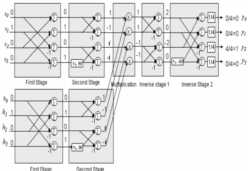
Figure 3. Flow diagram for cyclic convolution - N=4.

It is possible to appreciate in Figure 3 the stages of the algorithm. For N 22, the algorithm shows

2 log₂

1 N

S stages of multiplication by the roots of the polynomial _z41

. We can observe also 2

log₂

2 N

S stages that are similar to the process for the inverse Fourier transform, and one multiplication stage of the “transformed” sequences of sizeN 4. The total numbers of operation are 4 multiplications and 24 sums. A similar process to the one described above is done with the roots of the polynomial N 1

z , for

(8)

The general algorithm uses a field of constants that are organized according to its use in the mapping of the convolution process. Figure 4 below shows an easy manner to find constants for different order sequences.

Figure 4. Roots of unit for different order sequences.

Now, the mathematical foundation for the algorithm is described by means of a general example; consider

) 1 (4

) ( ) ( ) (

z

z h z x z

y for the polynomials:

3 3 2 2 1 0

)

(z x xz x z xz

x

3 3 2 2 1 0

)

(z h hz h z hz

h

3 1 2 2 1 3 0

0

)

(z xh xh xh xh y

(x₁h₀x₀h₁x₃h₂x₂h₃)z

3 3 0 2 1 1 2 0 3

2 3 3 2 0 1 1 0 2

) (

z h x h x h x h x

The above product can be computed, by direct computation, using 16 multiplications and 12 sums. By means of the Chinese remainder theorem this polynomial product can be realized following three steps:

1) The two polynomials are divided way long division by the roots of the monic polynomial (_z41)

obtaining the following remainders: )

(x₀x₁x₂x₃ and (h₀h₁h₂h₃) for (z1)

)

(x₀x₁x₂x₃ and (h₀h₁h₂h₃) for (z1)

)

(x₀ix₁x₂ix₃ and (h₀ih₁h₂ih₃) for (zi)

)

(x₀ix₁x₂ix₃ and (h₀ih₁h₂ih₃) for (zi)

2) Now, by multiplying those remainders we can obtain:

1

m (x₀x₁x₂x₃)(h₀h₁h₂h₃)/2

2

m (x₀x₁x₂x₃)(h₀h₁h₂h₃)/2

3

m (x₀ix₁x₂ix₃)(h₀ih₁h₂ih₃)/2

4

m (x₀ix₁x₂ix₃)(h₀ih₁h₂ih₃)/2 3) By means of a linear combination we obtain:

2 / )

( ₁ ₂ ₃ ₄

0 m m m m

y

2 / ) / ) (

)

(( 1 2 3 4

1 m m m m i

y

2 / )) (

)

(( ₁ ₂ ₃ ₄

2 m m m m

y

2 / ) / ) (

)

(( 1 2 3 4

3 m m m m i

y

The great advantage of the matrix representation proposed in this paper is that it is not necessary to

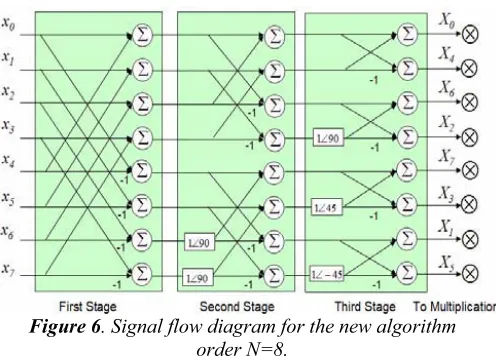
calculate the polynomials remainders. Other minimal multiplicative complexity algorithms based on CRT such as Winograd’s algorithms need to realize this decomposition. For this reason, the whole algorithm complexity is reduced. It is very interesting to compare the new algorithm with those that use the DFT to compute cyclic convolution. The pre-Hadamard stages are compared in Figure 4 and Figure 5 forN 8.

A comparison between theses figures shows a high correlation in the mapping of the two algorithms into a signal flow diagram. Even though their signal flow diagrams are slightly different, the two figures show the same number of computations (O(Nlog(N)). An advantage of the present algorithm, is that it does not need a stage of bit reversal operation. For this reason, this will improve the time necessary to realize the convolution operation with respect to the radix 2 and radix 4 FFT approaches. This is due to the fact that they need to do twice this process (at the beginning and in the post Haddamard multiplication) in order to obtain the output data in the required organized manner.

Figure 5. Signal flow diagram for FFT-2 order N=8.

Figure 6. Signal flow diagram for the new algorithm order N=8.

IV. CONCLUSION

(9)

The principal goal was to obtain a recursive algorithm, easy to implement, with the advantage of not needing to realize the polynomial divisions by the roots of unity in order to obtain less number of multiplications. The algorithm was also compared with the algorithm that uses the Fourier transform approach and the present algorithm has the comparative advantage that it does not require to realize the bit reversal operation in order to exhibit an in-place computation.

This work changes the conceptual framework of the computation of the CC using the FFT and locates it in a structure of minimum mathematical complexity. The algorithm obtained is limited to polynomials with length a power of 2, and its flow diagram suggests the possible use of Kronecker or Tensor products as a tool to improve their performance by means of parallel processing.

Future work includes the use of the methodology employed here for the problem of 2 dimensional cyclic convolution operations, and the mapping to parallel hardware structure by use of VHDL and low power complex multiplication operations.

ACKNOWLEDGMENT

The authors would like to thank Dr. Shmuel Winograd for his helpful suggestions and comments during the design and development stages of this work.

REFERENCES

[1] H. Krishna, B. Krishna, K. Y. Lin, J. D. Sun,

Computational Number Theory and Digital Signal Processing (CRC Boca Raton, Florida, 1994).

[2] Abraham H. Díaz-Pérez, Análisis y Diseño de Algoritmos Para la Computación con Estructuras Circulantes, MS Thesis, ECE Dept., UPRM, Mayagüez, Puerto Rico, May 2004.

[3] D. Chiper, M.N.S. Swamy, M. Omair Ahmad, “An Efficient Unified Framework for Implementation of a Prime-Length DCT/IDCT with High Throughput,” IEEE Trans. on Signal Processing, vol. 55, no. 6, June 2007. [4] C. Cheng, K. K. Parhi, “Low-Cost Fast VLSI Algorithm for Discrete Fourier Transform,” IEEE Trans. on Circuits and Systems, vol. 54, no. 4, April 2007. [5] C. Cheng, K. K. Parhi, “Hardware Efficient Fast DCT Based on Novel Cyclic Convolution Structures,” IEEE Trans. On Signal Processing, vol. 54, no. 11, Nov. 2006. [6] Y. Guo, J. Zhang, D. McCain, J. R. Cavallaro, “Structured Parallel Architecture for Displacement MIMO Kalman Equalizer in CDMA Systems,” IEEE Trans. on Circuits and Systems, vol. 54, no. 2, Feb. 2007.

[7] H. Zhang, M. Xia, G. Hu, “A Multiwindow Partial Buffering Scheme for FPGA-Based 2-D Convolvers,”

IEEE Trans. on Circuits and Systems, vol. 54, Feb. 2007. [8] D. Zhu, Z. Zhu, “Range Resampling in the Polar Format Algorithm for Spotlight SAR Image Formation Using the Chirp z-Transform,” IEEE Trans. on Signal Processing, vol. 55, no. 3, March 2007.

[9] D. G. Myers, Efficient Convolution and Fourier Transform Techniques (Prentice Hall, Australia, 1990). [10] K. Hoffman, R. Kunze, Linear Algebra, (Prentice Hall, Inc. , New Jersey, 1961.

[11] D. Rodriguez, Computational Signal Processing and Sensor Array Signal Algebra: A Representation Development Approach, Book Draft, (UPRM, PR, 2002). [12] J. Davis, Circulants Matrices (John Wiley, New York, 1979).

[13] J. McClellan and C. Rader, Number Theory in Digital Signal Processing. Englewood Cliffs, NJ: Prentice Hall 1979.

[14] S. Winograd, Arithmetic complexity of computations

(Society for Industrial and Applied Mathematics, 1980).

[15] M. Heideman, Multiplicative complexity, convolution, and the DFT (Springer Verlag, New York 1988)

[16] J. Cooley, Some applications of computational complexity Theory to Digital Signal Processing. 1981 Joint Automatic Contr. Conf. University of Virginia, June 17-19 1981.

Abraham H. Diaz-Perez was born in Barranquilla-Colombia. He received the B.S. in Electrical Engineer degree from the Technologic University of Bolivar at Cartagena-Colombia in 1997 and the M.Sc. in Electrical Engineer from the University of Puerto Rico at Mayaguez-Puerto Rico in 2004. He is currently working in the Popular University of the Cesar at Valledupar-Colombia, the work fields cover fast algorithms for multidimensional cyclic convolution, adaptive filter theory and acoustic and image processing applications. Prof. Diaz-Perez is an international judge for different IEEE conferences as MWCASS and IASTED, and he is recipe of different grants as the PR Louis Stroke Alliance for Minorities Participation and Colciencias.

Cyclic Convolution Algorithm Formulations Using Polynomial Transform Theory