Ashish et al. World Journal of Engineering Research and Technology
APPROXIMATE, GENERALIZED FIELD DATA BASED
MATHEMATICAL MODELING AND ANN SIMULATION OF PVC
PIPE MANUFACTURING PROCESS
Ashish D. Vikhar*1 and J.P. Modak2
1
Ph.D. Research Scholar, SGB Amravati University, Amravati, Maharashtra, India.
2
Emeritus Professor in Mechanical Engineering, AICTE Emeritus Fellow and Dean
(Research & Development), Priyadarshini College of Engineering, CRPF Campus, Hingna
Road, Nagpur, Maharashtra, India.
Article Received on 20/05/2015 Article Revised on 12/06/2015 Article Accepted on 04/07/2015
ABSTRACT
PVC pipe extrusion with single screw extruder is the most widely used
process among small and medium sized manufacturing industries in
India. The increasing importance of plastic extrusion is gaining new
dimensions in the present industrial age. This paper shows an idea
about the methodology of formulation of field data based mathematical
model for the dependent process parameters (ΠD1), pipe dimensions
(ΠD2), pipe weight (ΠD3) and productivity (ΠD4) during PVC pipe
manufacturing process. It helps to develop an approximate, generalized but reliable model for
predicting and optimizing the critical process parameters which affects the quality,
productivity of the process. This paper presents the procedure to analyze the impact of field
parameters on the performance of PVC pipe manufacturing process. At the end of this work,
the findings indicate that the topic under study is of good importance, as no such approach of
formulation field data based mathematical models and simulation is adopted for small scale
industries engaged in PVC pipe manufacturing.
KEYWORDS: Artificial neural network, field data based mathematical models, PVC pipe extrusion.
*Correspondence for Author
Ashish D. Vikhar Ph.D. Research Scholar,
SGB Amravati University,
Amravati, Maharashtra,
India.
World Journal of Engineering Research and Technology
WJERT
BACKGROUND
In present scenario of Indian manufacturing it is found that most of the small and medium
scale manufacturer‟s in the field of manufacturing of PVC pipes are using non-standardized
methods to produce PVC pipes. Some of these manufacturers are also located at the area of
Maharashtra Industrial Development Corporation (MIDC) of rural regions as well as few at
urban regions. It is observed through the field study that such manufacturer‟s do not seriously
bothers about performance evaluation terms viz. quality, productivity, optimization, cycle
time reduction and others. Such manufacturer‟s just wants to produce their PVC pipes and to
sale it into the market at low costs. Because of the low cost, these pipes are seen in big
demand of purchase by the poor, uneducated farmers and such other customer‟s. But after
some use of such low quality pipes the customer‟s in said category felt unsatisfied with the
problems viz. poor quality and poor performance of the pipes. To overcome these problems
the methodology of formulation of field data based mathematical models is supposed to be
found fit to produce the optimal type of quality pipes with optimal process parameters and at
optimal productivity. For this purpose some small scale industries in these sectors are visited
and the detailed study is performed regarding the entire operation of PVC pipe manufacturing
process executed at their plants. It is studied that majority of total operation are executed
manually and on the basis of trial-error approach. This needs to be focused and develop a
mathematical relation which simulate the real input and output data.
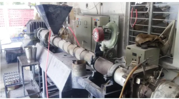
Introduction to PVC pipe extrusion using single screw extruder
In the extrusion of plastics (figure 1), raw thermoplastic material in the form of small beads is
gravity fed from a top mounted hopper into the barrel of the extruder. Additives such as
colorants and UV inhibitors are often used and can be mixed into the main material prior to
arriving at the hopper. The material enters through the feed throat (a funnel shaped opening
near the rear of the barrel) and comes into contact with the screw. The rotating screw (at
around 120 rpm) forces the plastic beads forward into the barrel which is heated to the
desired melt temperature of the molten plastic (usually around 200°C). In most processes, a
heating profile is set for the barrel in which three or more independently controlled heaters
gradually increase the temperature of the barrel from the rear (where the plastic enters) to the
front. In most extruders, cooling fans are present to keep the temperature below a set value if
too much heat is generated. This extrusion process continues till the die. The die is an upright
cylinder with a circular opening similar to a pipe die. The diameter can be a few centimeters
Figure 1:PVC pipe extrusion process
Approach of formulation of field data based mathematical model
To start let us assume that the observed phenomenon has four inputs A, B, C, and D. the
responses are Y1 and Y2. It is intended to establish the mathematical relationships in much
generalized form as under.
Y1 = K1 [(A) a1, (B) b1, (C) c1, (D) d1] ………… (1) Y2 = K2 [(A) a2, (B) b2, (C) c2, (D) d2]………… (2)
This is known as exponential form of the model. Assuming such a form, it is convenient to
decide precisely the degree of influence of one input relative to other inputs on the response
variable.[2] After having established this, one would be able to decide the inputs which have low influence on the response. Thus this aspect will crystallize the inputs which need
attention from the point of view of improving the methods of performing the activity. This is
the main purpose of formulation of FDBM for a process. Recalling equations (1) and (2) all
needs to be done is to decide 5 unknown in this equation viz. k1, a1, b1, c1 and d1. For this
purpose we need only 5 observations. Let us select observation number 1,23, 35, 41 and 48
(out of 50 valid sets of readings) then all this observations values of Y,A,B,C,D are known.
As an example for observation 23, may be denoted as Y (23), A (23), B (23), C (23), D (23),
then if we substitute these values in equation (1)
Y1 (23) = k1 [(A23) a1, (B23) b1, (C23) c1, (D23) d1] …… (3)
Taking log on both sides, following log linear relation can be obtained.
For observation number 1, 35, 41 and 48 similar equation can be formed. This gives a system
set of 5 equations which can be put in matrix from as under
Log Y1 (1) = 1 log (A1) log (B1) log (C1) log (D1) log k1
Log Y1 (23) = 1 log (A23) log (B23) log (C23) log (D23) a1
Log Y1 (35) = 1 log (A35) log (B35) log (C35) log (D35) b1 … (5)
Log Y1 (41) = 1 log (A41) log (B41) log (C41) log (D41) c1
Log Y1 (48) = 1 log (A48) log (B48) log (C48) log (D48) d1
In equation (5) all quantities are known excepting logk1, a1, b1, c1, d1. It is recommended to
use MATLAB software for this purpose for making this process of model formulation less
cumbersome. If equation (5) is expressed as b=Ax, then to get elemental values in vector x
MATLAb-7 allows an operator called „left division‟. In particular, the command x=A\b
solves the matrix equation b=Ax. Thus, K1, a, b1, c1, and d1 can be found for one set of 5
readings from the total set of observation taken. Thus if 50 observation are taken then one
will arrive at NCR combinations. Here 50C5 will be combination of 50 observations taken
any 5 at a time. This will result in 2, 118, 760 possible combinations. Thus arithmetic average
of these would probably be the most reliable values of k1, a1, b1, c1 and d1. After
completing this laborious task the exact form of model will be obtained.
Formulation of field data based mathematical model
When one is studying any completely physical phenomenon but the phenomenon is very
complex to the extent that it is not possible to formulate a logic based model correlating
causes and effects of such a phenomenon, then one is required to go in for the field data
based models.[1] In view of the dynamic nature of the context under investigation (which reveals complex phenomenon), it is decided that to formulate a field data based models for
dependent process parameters (ΠD1), pipe dimensions (ΠD2), pipe weight (ΠD3) and
productivity (ΠD4). These models are established adopting methodology of
experimentation.[5] It is planned to collect the data by taking extensive observations in the process of PVC pipe extrusion process by actually visiting and PVC pipe manufacturing
industries. The planning is carried out by using the classical plan of experimentation [6]. The
response data is collected based on the entire generalized models. The approach adopted for
formulating approximate, generalized field data based mathematical model suggested by
independent and dependent variables or quantities. (2) Reduction of independent variables
adopting dimensional analysis. (3) Formulation of the model.
Identification of variables and its dimensional analysis
Any physical quantity prevailing in the process under study is designated as process
variable.[5] Process variables are categorized as: 1) Independent variables, 2) Dependent variables and. The following process variables are identified and they are grouped in
dimensionless pi terms in table 1.
Table 1:Identification of variables and pi terms
Pi term Code Description of Pi terms Pi term equation
Π1 C6 Acceleration due to gravity mm/s2
C3 Distance of electric motor from the extruder
C2 Mass or weight of the electric motor (kg)
C5 Torque on electric motor (N-mm)
Π2 A12 Weight of extruder machine (kg)
x
x
x
A5 Hopper capacity (kg)
A1 Extruder machine length (mm)
A2 Extruder machine width (mm)
A3 Extruder machine height (mm)
A4 Barrel centerline from floor (mm)
A7 Screw outside diameter (mm)
A8 Screw inside diameter (mm)
A6 Hopper height (mm)
A9 Screw pitch (mm)
A10 Barrel length (mm)
A11 Barrel diameter (mm)
A14 Die length (mm)
A13 Die diameter or size (mm)
Π3 W1 Resin wastage (kg)
x
x
W2 Dust (kg)
W3 Filter (gm))
W4 Chemical wax (gm)
W5 TBLS powder (gm)
W6 Steric acid (gm)
W7 Wastage raw material size (mm)
W8 Powder size (mm)
W9 Filter material size (mm)
ΠD1 D1 Screw speed (m/s)
D2 Melt viscosity (N-s/m2) or (kg/m-s)
D3 Melt density (kg/m3)
D4 Extruder pressure (kg/ms2)
D6 Extruder temperature (0C)
ΠD1= x
x
D7 Die temperature (0C)
D8 Pipe diameter or size (mm)
D9 Pipe wall thickness (mm)
D10 Pipe weight (kg)
D11 Processing time (sec)
D12 Productivity
ΠD2 P1 Pipe diameter (mm)
ΠD2 =
P2 Pipe wall thickness (mm)
ΠD3 Y1 Pipe weight (kg)
ΠD3 = Y1
Y2 Processing time (sec)
ΠD4 T2 Productivity ΠD4 = x Y2/Y1
Dimensional analysis is the best known and the most powerful technique of reducing the
number of variables and making the experimental plan compact without loss of generality or
control.[3] Dimensional analysis, basically, helps in deciding algebraic relationship amongst the various physical quantities encountered in the process.[4] Using Buckingham π theorem following dimensional equation is formed. Three independent pi terms (Π1, Π2, Π3,) and
four dependent pi terms (ΠD1, ΠD2, ΠD3, ΠD4,) have been in the design of experimentation and are available for the model formulation. Independent Π terms = (Π1, Π2, Π3), Dependent Π terms = (ΠD1, ΠD2, ΠD3, ΠD4,). Each dependent Π is assumed to be function of the available independent Π terms,
For Process Parameters (ΠD1), ΠD1 = k1 x (Π1) a1
x (Π2) b1 x (Π3) c1 --- (6)
For Pipe Dimensions (ΠD2), ΠD2 = K2 x (Π2) a2
x (Π2) b2 x (Π3) c2 --- (7) For Pipe Weight (ΠD3), ΠD3 = k3 x (Π3) a3 x (Π3) b3
x (Π3) c3 --- (8) For Productivity (ΠD4), ΠD4 = k4 x (Π4) a4
x (Π4) b4 x (Π4) c4 --- (9)
By adopting the approach given above, the field data based mathematical models are
formulated as given below
(1)
(2)
(3)
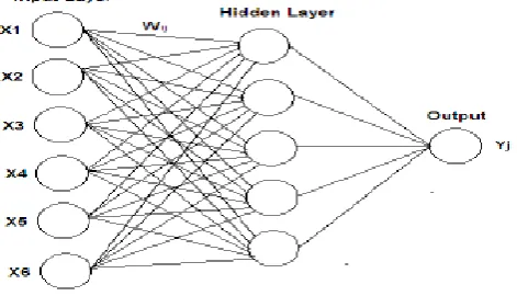
Artificial Neural Network (ANN) based simulation
Artificial neural networks (ANN) can replicate numerous functions of human behavior,[6] which are formed by a predetermined number of layers with altered computing elements
called neurons. In order to build a network, the neurons are interrelated. The crowd of
connections determines the form and objectives of the ANN.[7] The processing capacity of the network is stored in the inter unit connection strengths, or weights, which are tuned in the
learning process.
Figure 2: Basic structure of ANN 6/5/1 network
The various steps[7][8] followed in developing the algorithm to form ANN are: (1) The observed data from the experimentation is separated into two parts viz. input data or the data
of independent pi terms and the output data or the data of dependent pi terms. The input data
and output data are imported to the program respectively. (2) The input and output data is
read by prestd function and appropriately sized. (3) In preprocessing step the input and output
data is normalized using mean and standard deviation. (4) Looking at the pattern of the data,
feed forward back propagation type neural network is chosen. (6) This network is then
trained using the training data. The computation errors in the actual and target data are
computed and then the network is simulated. In this work the main issue is to predict the
future result. In such complex phenomenon involving non-linear system it is also planned to
develop Artificial Neural Network (ANN). The output of this network can be evaluated by
comparing it with observed data and the data calculated from the mathematical models. For
development of ANN the designer has to recognize the inherent patterns.[9] Once this is accomplished training the network is mostly a fine-tuning process.[10] Following graphs shows the comparison and neural network predictions for all four models
1 2 3 4 5 6 7 8 4
4.5 5 5.5 6 6.5 7
Experimental
Comparision between practical data, equation based data and neural based data Practical Equation Neural
Figure 3: Comparison of results of experimental, model and ANN for model 1.
1 2 3 4 5 6 7 8
4 4.5 5 5.5 6 6.5 7
Experiment No.
Ou
tpu
t
Output (Red) and Neural Network Prediction (Blue) Plot Experimental Neural
Figure 4: Neural network predictions for model 1.
For model 2:
1 2 3 4 5 6 7 8
45 50 55 60 65
Experimental
Comparison between practical data, equation based data and neural based data
Practical Equation Neural
Figure 5:Comparison of results of experimental, model and ANN for model 2.
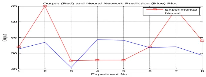
1 2 3 4 5 6 7 8
45 50 55 60 65
Experiment No.
Ou
tpu
t
Output (Red) and Neural Network Prediction (Blue) Plot Experimental Neural
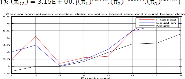
For model 3:
1 2 3 4 5 6 7 8
2.5 3 3.5 4 4.5 5 5.5 6 6.5 Experimental
Comparison between practical data, equation based data and neural based data
Practical Equation Neural
Figure 7: Comparison of results of experimental, model and ANN for model 3.
1 2 3 4 5 6 7 8
2.5 3 3.5 4 4.5 5 5.5 6 6.5 Experiment No. Ou tpu t
Output (Red) and Neural Network Prediction (Blue) Plot
Experimental Neural
Figure 8: Neural network predictions for model 3.
For model 4:
1 2 3 4 5 6 7 8
0.03 0.035 0.04 0.045 0.05 0.055 0.06 0.065 0.07 0.075 Experimental
Comparision between practical data, equation based data and neural based data
Practical Equation Neural
Figure 9: Comparison of results of experimental, model and ANN for model 4.
1 2 3 4 5 6 7 8
0.03 0.035 0.04 0.045 0.05 0.055 0.06 0.065 0.07 0.075 Experiment No. Ou tpu t
Output (Red) and Neural Network Prediction (Blue) Plot
Experimental Neural
CONCLUSION
Most of the owners of small scale manufacturer‟s of PVC pipe manufacturing firms are not
aware as to what extent the relationship exists between various inputs of PVC pipe
manufacturing process. This can be achieved through formulation of field data based
mathematical modeling. From the results it is seen that the mathematical models can be
successfully used for the computation of dependent terms for a given set of independent
terms. The mathematical model formulated is used to analyze the data and to establish
relationship between different variables of PVC pipe manufacturing process. From ANN
simulation modeling “Intensity of interaction of inputs on deciding Response “can be
predicted which will help to control the variable for the desired results.
REFERENCES
1. Spiegel, M. R. 1998. Theory and problems of problems of probability and statistics,
Schaum Outline series, Mc Graw-Hill Book Company.
2. Hilbert Schenck Junior, Theory of Engineering Experimentation, McGraw Hill, New
York (1961).
3. Modak J. P., “A Specialized course on Research Methodology in Engineering and
Technology”, at Indira college of Engineering and Management, Pune (India), during
12th to 14th March, 2010.
4. Modak, J. P. &Bapat, A. R., “Formulation of Generalized Experimental Model for a
Manually Driven Flywheel Motor and its Optimization”, Applied Ergonomics, U.K.,
1994; 25(2):119-122.
5. Modak, J. P. & Bapat, A. R., “Formulation of Generalized Experimental Model for a
Manually Driven Flywheel Motor and its Optimization”, Applied Ergonomics, U.K.,
1994; 25(2):119-122.
6. A. R. Lende, “Modelling of pedal driven flywheel motor by use of ANN”, M. Tech.
Thesis, PCE, Nagpur.
7. S. N. Shvanandam, “Introduction to Neural Network using Matlab 6.0”, McGraw Hill
publisher.
8. Stamtios V. Kartaplopoulos, Understanding Neural Networks and Fuzzy Logics, IEEE
Press.
9. Neural Network Toolbox TM 7 User‟s Guide R2010a, Mathworks.com.