Learning a Classication-based Glioma Growth Model Using MRI Data

Learning a Classification-based Glioma Growth

Model Using MRI Data

Marianne Morris

_{, Russell Greiner}

_{, J¨org Sander}

_{, Albert Murtha}

_{, and Mark Schmidt}

_{Department of Computing Science, University of Alberta,}

Edmonton, AB, T6G 2E8, Canada

{

marianne, greiner, joerg, schmidt

}@cs.ualberta.ca

2

_{Department of Radiation Oncology, Cross Cancer Institute,}

11560 - University Ave, Edmonton, AB, T6G 1Z2, Canada

Abstract— Gliomas are malignant brain tumors that grow by invading adjacent tissue. We propose and evaluate a 3D classification-based growth model, CDM, that predicts how a glioma will grow at a voxel-level, on the basis of features specific to the patient, properties of the tumor, and attributes of that voxel. We use Supervised Learning algorithms to learn this general model, by observing the growth patterns of gliomas from other patients. Our empirical results on clinical data demonstrate that our learnedCDMmodel can, in most cases, predict glioma growth more effectively than two standard models: uniform radial growth across all tissue types, and another that assumes faster diffusion in white matter. We thoroughly study CDM results numerically and analytically in light of the training data we used, and we also discuss the current limitations of the model. We finally conclude the paper with a discussion of promising future research directions.

Index Terms— machine learning, brain tumors, glioma, growth models, prediction

I. INTRODUCTION

Primary brain tumors originate from a single glial cell in the nervous system, and grow by invading adjacent cells, often leading to a life-threatening condition. Proper treatment requires knowing both where the tumor mass is, and also where the occult cancer cells have infiltrated in nearby healthy tissue. Some conventional treatments implicitly assume the tumor will grow radially in all directions — e.g., the standard practice in conformal

radiotherapy involves irradiating a volume that includes both the observed tumor, and a uniform 2cm margin around this border [11], [12]. Swanson’s model [27] claims the tumor growth rate is 5 times faster in white matter, versus grey matter. Our empirical evidence, how-ever, shows that neither model is particularly accurate.

We present an alternative approach to modeling tumor growth: use data from a set of patients to learn the

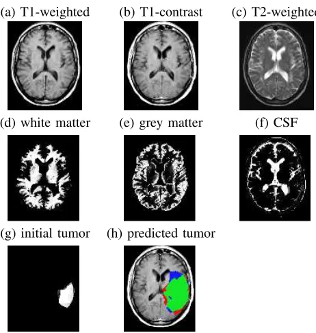
parameters of a diffusion model. In particular, given properties of the patient, tumor and each voxel (based on MRI scans; see Fig. 1(a–g)) at one time, our CDM system predicts the tumor region at a later time (Fig. 1(h)). This model can help define specific treatment boundaries that would replace the uniform, conventional 2cm margin. It can also help find regions where radiologically occult cancer cells concentrate but do not sufficiently enhance

on the MRI scan. Therefore, the model can help make radiotherapy more effective by specifying the treatment volume more precisely, which would allow doctors to apply a higher radiation dose. This will help eradicate the diffuse glioma cells in surrounding tissue, which will reduce the possibility of recurrence while minimizing the amount of healthy tissue compromised.

Section II overviews and discusses standard glioma dif-fusion models. Section III briefly presents the framework of the proposed model,CDM. Section IV formally defines the diffusion models we are considering. Section V then describes our experiments that test our CDM model, and compares its performance with two other models, based respectively on na¨ıve uniform growth and on tissue-based diffusion. Finally, Section VI concludes the paper by discussing the future research directions that we are con-sidering to extend our current model. Additional details are in [1], [19], [20].

II. RELATEDWORK

In recent decades, glioma growth modeling has offered important contributions to cancer research, shedding light on tumor growth behavior and helping improve treatment methods. Earlier tumor growth models were simply based on exponential growth, and were later modified to account for the gradual slow down as the tumor size becomes larger [21]. Recent models are more sophisticated and take as parameters the heterogeneity of glioma cells and the brain anatomy. In this section, we describe two types of tumor modeling: volumetric at the macroscopic level, and models based on white matter invasion.

A. Macroscopic and Volumetric Modeling

In this section, we discuss the traditional framework in predicting glioma diffusion using growth and proliferation parameters. We review three of these models:

Kansal et al. [14] simulate the gompertzian growth,

which views the tumor as a population of cells and the growth as a dynamic process where proliferating and inactive classes of cells interact. Kansal et al. use

(a) T1-weighted (b) T1-contrast (c) T2-weighted

(d) white matter (e) grey matter (f) CSF

(g) initial tumor (h) predicted tumor

Figure 1. Axial slices of brain tumor patient: (a) T1-weighted scan; (b) T1-weighted scan after injecting the patient with gladolinium con-trast; (c) T2-weighted scan; (d) white matter (of this patient); (e) grey matter; (f) CSF — cerebrospinal fluid; (g) segmented patient tumor; (h) predicted patient tumor, after adding30,000voxels in 3D, overlayed on T1-contrast (green represents the true positives, red the false positives and blue the false negatives).

cells, from dividing cells at the periphery, through non-proliferating, and finally to the necrotic state at the centre of the tumor. This model is designed to predict the growth of glioblastoma multiforme (GBM), the most aggressive, gradeIVgliomas. The model does not account for various tumor grades, brain anatomy, nor the infiltrating action of cancer cells in tissue near the tumor.

Tabatabaiet al.[30] simulate asymmetric growth as in

real tumors and accommodate the concept of increasing versus decreasing tumor radii (due to treatment effects), but do not account for various clinical factors involved in malignant diffusion. Instead, their model describes tumors as self-limited systems, not incorporating the interactions between healthy and cancer cells at the tumor border and the competition of cells inside the tumor. This has not proven to be a realistic representation of clinical cancer diffusion.

Zizzari’s model [32] describes the proliferation of GBMs using tensor product splines and differential equa-tions, the solutions of which give the distribution of tumor cells with respect to their spatio-temporal coordinates. Zizzari extends his growth model to introduce a treatment planning tool that incorporates a supervised learning task. However, his growth predictions are based only on geometric issues, and do not consider biological factors nor patient information.

B. Glioma Modeling based on White Matter Invasion

The trend in glioma research is to study biological and clinical factors involved in cancer diffusion through

healthy tissue. Recent models provide a more promising direction, which can also help provide more effective treatment. In this section, we review models that incor-porate the heterogeneity of brain tissue and histology of cancer cells.

Swanson et al. [27] develop a model based on the

differential motility of glioma cells in white versus grey matter, suggesting that the diffusion coefficient in white matter is 5 times that in grey matter. This model was extended to simulate virtual gliomas [29] and to assess the effectiveness of chemotherapy delivered to different tissue types in the brain [28]. This modeling is different from ourCDMsystem as we do nota prioriassume the cancer

diffusion rates in different tissue types, but rather our system canlearnglioma diffusion behavior from clinical

data.

Price et al.[24] use T2-weighted scans and Diffusion

Tensor Imaging1 _{(DTI) to determine whether DTI can} identify abnormalities on T2 scans. Regions of interest particularly include white matter adjacent to the tumor, and areas of abnormality on DTI that appear normal on T2 images. Results demonstrated further glioma invasion of white matter tracts near the observed tumor. Our learning system has the potential of finding just such behavior.

Clatz et al. [7] propose a model that simulates the

growth of GBMs based on an anatomical atlas that includes white fibre diffusion tensor information. The model is initialized with a tumor detected on the MRI scan of a patient, and results are evaluated against the tumor observed six months later. However, model results are reported for only one patient, leaving in question how it performs on a variety of patients, and with various tumor types. Our model, on the contrary, is learned from a number of patients with various tumor types and from various age categories.

C. Discussion

Each of the glioma diffusion models presented above describes the geometrical growth of gliomas as evolving objects. Few of these models use the biological com-plexity of cancerous tumors, the heterogeneity of the human brain anatomy, or the clinical factors of malignant invasion. Moreover, none of these earlier systems attempts tolearn general growth patterns from existing data, nor

are they capable of predicting different growth patterns for different tumor grades (as opposed to methods specifically designed to predict GBM growth only).

The literature does suggest that the following factors should help us predict how the tumor will spread —i.e.,

whether the tumor is likely to infiltrate to a new voxel:

Anatomical features of the brain: regions that

rep-resent pathways versus brain structures that act as boundaries to the spreading action of the malignant cells.

Properties of the tumor: the grade of the tumor (as

high-grade gliomas grow much faster than low-grade ones); the location of the tumor within the brain (as the shape of the tumor depends on surrounding anatomical structures).

Properties of the voxels(at the periphery of the tumor

where there can be interaction between malignant and normal cells): its tissue type — grey versus white matter; whether it currently contains edema2_. We incorporate these diffusion factors as learning features into our ‘general’ diffusion model, CDM. The remainder of this paper describes the diffusion models we implemented, presents the experiments, and evaluates the performance of the three models given our dataset of MRI scans.

This paper extends [20] as follows: We describe the model framework and the processing techniques applied to the MRI scans. We further explain CDM results and thoroughly study the tumor growth behavior learned by our model. We also evaluate the training data, the per-formance of the classifiers we used in the experiments, and the fairness of performance measures in light of the challenges and data limitations. In addition, we discuss current model limitations, and we describe our current work and ongoing experiments. Finally, we discuss sev-eral promising research ideas that we intend to incorporate in our current model.

In the following section, we describe how we processed the MRI scans in order to be able to use this data in the experiments. In Section IV, we describe the implementa-tion of the growth models we developed.

III. MODELFRAMEWORK

In this section, we briefly describe the preprocessing techniques and steps we applied to the MRI scans in order to be able to extract the learning features from the images.

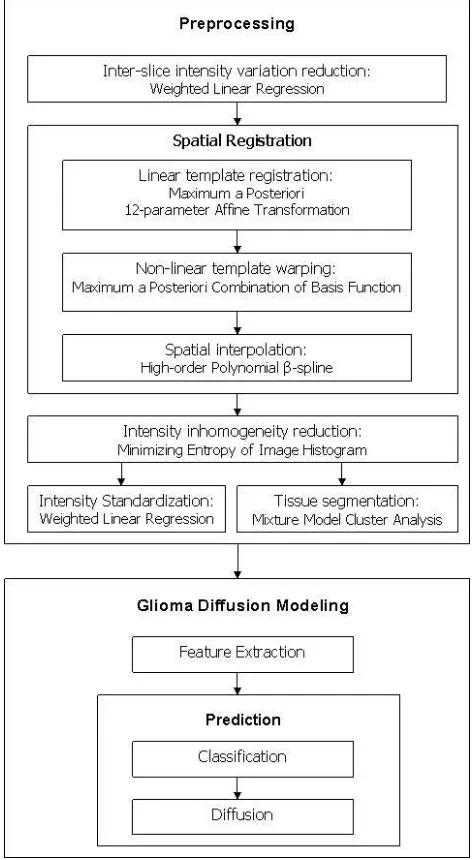
Noise Reduction: We reduce inter-slice intensity

variations (which are sudden changes in the intensity values across consecutive slices of a scan) by apply-ing a weighted least squares estimation method [25]. We also reduce intensity inhomogeneity (a slowly varying spatial field across the scan, inherent to MR) with the help of SPM [5].

Registration: We use SPM to linearly register and

then non-linearly warp all patients’ scans to a stan-dard coordinate system (a template) [2], [3]. Here, we use the Colin Holmes [13] and ICBM3 _[9] tem-plates (see Fig. 4). After linear registration and non-linear warping, we use SPM to spatially interpolate the brain and tumor volumes, which fills the inter-slice gaps producing8mm3 voxels.

Intensity Standardization: We use a weighted linear

regression method [25] to reduce the intensity

differ-2_{Swelling due to accumulation of excess fluid.}

3_{The International Consortium for Brain Mapping, formed in 1993,} has the primary goal of continuing to develop a probabilistic reference system for the human brain.

Figure 2. Overview ofCDMframework. The framework of the proposed model,CDM, consists of two main components: the preprocessing of the MRI scans and the prediction of glioma growth.

ences among the various scans as some scans appear relatively brighter or darker than others.

Tissue Segmentation: We differentiate between the

grey matter, white matter, and CSF of a patient or of the template with the use of SPM [2], [4], [5] (see Fig. 1(d-f) for an illustration of tissue segmented with SPM).

The model framework consists of two main components: the preprocessing of the MRI scans and the prediction of tumor growth — as shown in Fig. 2. Additional details about the algorithms used in processing the MRI scans are in [19].

IV. DIFFUSIONMODELS

1. Diffusion(VoxelLabel: VL; GeneralInfo: e; int: s)

%VL[i, j, k]=1 if positionhi, j, kiis a tumor % Initially VLcorresponds to current tumor

% When algorithm terminates,VLwill correspond to tumor containing “s” additional voxels 2. total count := 0

done := false

3. Do forever:

4. ComputeN :=



  

  

hx, y, zi

VL[x, y, z] = 0 & W 

  

VL[x+ 1, y, z] = 1 _∨ VL[x₋1, y, z] = 1 _∨

.. .

VL[x, y, z₋1] = 1 

  



  

   5. For each locationvi∈N

6.

Determine if

v

becomes a tumor

8. SetVL[vi] := 1

9. total count++;

10. If (total count ==s), return

Figure 3. Generic Diffusion Model

a tumor and “0” otherwise (see Fig. 1(g))4 _{as well as} general informatione=e_{P atient∪}e_{T umor∪ {}e_i}i about the patiente_{P atient}, the tumore_{T umor}and the individual voxelse_i(see Section IV-A). The third input is an integer

s that tells the diffusion model how many additional

voxels to include. See line 1 of Fig. 3. The output is the prediction of the next sadditional voxels that will be

incorporated into the tumor, represented as a bit-map over the image. For example, if the tumor is currently 1000 voxels and the doctor needs to know where the tumor will be, when it is 20% larger — i.e., when it is 1200

voxels — he would set s= 200.

A diffusion model first identifies the set of voxels N

just outside the border of the initial tumor; see line4 of Fig. 3. In the following diagram

v12 v11 v10 v9 v8

v1 v2 v6 v7 v5

X X v3 v4 X

X X X X X

(1)

(where eachXcell is currently a tumor),_N would consist of the voxels labeledv1through v5, but notv6norv7

(as we are not considering diagonal neighbors). Here,v8

through v12 are also not adjacent to the tumor voxels.

In the 3D case, each voxel will have 6 neighbors. The diffusion model then iterates through these candi-date voxels, vi∈N. If it decides that one has become a

tumor, it then updates VL (which implicitly updates the

tumor/healthy border) and increments the total number of “transformed voxels”; see lines 5−9 of Fig. 3. After processing all of these neighbors (in parallel), it will then continue transforming the neighbors of this newly enlarged boundary. If a voxel is not transformed on one iteration, it remains eligible to be transformed on the next iteration. When the number of transformed voxels matches the total s, the algorithm terminates, returning

the updatedVL assignment (Fig. 3, line10).

4_{Here, expert radiologists have manually delineated the “enhancing} regions” of tumors based on their MRI scans. Note this does not include edema, nor any other labels. We then spatially interpolate each patient image to fill inter-slice gaps and to obtain voxels of size 8mm3.

Figure 4. Spatial priors used in registration. Left to right: an example slice of each of the Colin Holmes template [13], and ICBM T1 and T2 average templates [9].

The various diffusion models differ only in how they determine if vi has become tumor — line 6 of Fig. 3.

The uniform growth model, UG, simply includes every

“legal” voxel it finds (where a voxel is legal if it is part of the brain, as opposed to skull, eye, etc.). The tissue-based model, GW, assumes the growth rate for white

matter is 5 times faster than for grey matter [27], and 10 times faster than other brain tissue. Here, whenever a neighboring voxel vi is white matter, it is immediately

included. If vi is grey matter (other tissue), its count

is incremented by 0.2 (resp., 0.1). GW does not allow diffusion into the skull. This is easy to determine as thee_i part of theGeneralInfoespecifies the tissue type of eachvivoxel, as computed by SPM [10] — see Fig. 1(d–

f).

A. CDMDiffusion Model

Our CDM model is more sophisticated. First, its deci-sion about each voxel depends on a number of features, based on:

the patient,e_{P atient}: the age (which may implicitly indicate the tumor grade).

the tumor, e_{T umor}: volume-area ratio, edema per-centage, and volume increase.

each individual voxel {e_i}i: various attributes for every voxel vi — spatial coordinates, distance-area

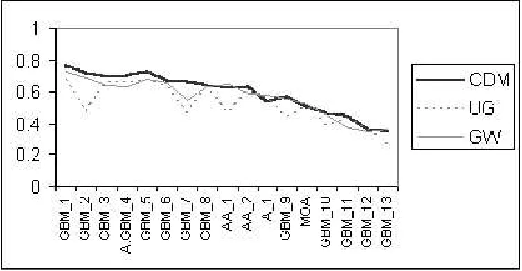
Figure 5. Empirical Results: The F-measure for the three Models with 17-fold “patient-level” (Note F-measure = precision = recall, for each patient — see Section V). Results correspond to the output of a logistic regression classifier, learned with feature setS1. The name of each patient identifies their tumor grades — Astrocytoma grade I (A) and grade II (A.GBM) that progressed into GBM, Mixed Oligo-astrocytoma grade II (MOA), Anaplastic astroyctoma grade III (AA), and the most common GBM.

both from the patient’s scan and a standard tem-plate5 _{[13] — after normalization and registration} using SPM [9]).

neighborhood of each voxel {e_{N ei}i}: attributes of each of the 6 neighbors of the voxel — whether a neighbor voxelnj is edema, white matter, grey

mat-ter, or CSF, and image intensities from the template’s T2 and T1-contrast.

(The webpage [1] provides more details about each of these features, as well as some explicit examples.)

CDM then uses a probabilistic classifier to compute the probability qi that one tumor neighbor vi of a

tu-mor voxel will become tutu-morous, qi = P_Θ(`(vi) =

Tumor|e_{P atient,}e_{T umor,}e_i), based on learned parame-tersΘ(see Section V). Some voxels can have more than one such tumor-neighbor;e.g., in diagram (1), the voxels

v1, v2andv5 each has a single tumor-neighbor, while v3 and v4 each has two. Each tumor-neighbor of the

voxel vi has a qi chance to transform this vi; hence if

there are k such neighbors, and each acts independently,

the probability thatviwill be transformed on this iteration

ispi= 1−(1−qi)k.CDMwill then transform this voxel

to be a tumor with probability pi. We then assign it to

be a tumor if pi > τ using a probability threshold of τ = 65%.6 CDMperforms these computations in parallel — hence on the first iteration, even ifv3is transformed, v4still has only two tumor-neighbors (on this iteration).

We discuss below howCDMlearns the parametersΘused inP_Θ(·).

5_{Several images of a normal brain of an individual, averaged and} registered to the same coordinate system.

6_{We experimented with several thresholds, and chose thisτ= 0.65} value as it provided the best observed accuracy.

V. EXPERIMENTS

We empirically evaluated the three models, UG, GW andCDM, over a set of 17 patients. For each patient, we had two sets of axial scansR₁ andR₂ taken at different

times, each with known tumor regions. Letsirefer to the

size of the tumor in scan Ri. For each patient, we then

input that patient’s initial scan (R₁) to each model, and

asked it to predict the nexts=s2−s1voxels that would be transformed. We then compare the predicted voxels with the truth —i.e., the tumor region of the second scan, R₂.

To measure the quality of each model, let “nt” be a set

of tumor cells for the patient that are actually transformed (i.e., this is the “truth”, associated withR₂) and “ptχ” be

the cells that theχmodel predicts will be transformed. We

then use the standard measures: “precision” ofχ(on this

patient) is |nt∩ptχ|

|ptχ| and “recall” is

|nt∩ptχ|

|nt_| . In our case,

as our diffusion models stop when|ptχ|=|nt|=s, the

precision and recall values will be the same7_{(see tables in} [1], [19]). We report results in terms of the “F-measure” = 2precisionrecall

precision₊recall [31], where F-measure = precision =

recall, for each patient.

While UG and GW are completely specified,CDMmust first be trained. We use a “patient level” cross-validation procedure: That is, we trained a learner (e.g., Logistic

Regression [17] or SVM [23]) on16patients, then tested on the 17th. Each training instance corresponded to a

single voxel vi around the initial tumor in the first scan R₁, with featurese_{P atient},e_{T umor}, ande_i, and with the label of “1” if this voxel was in the tumor in R₂, or

“0” otherwise. Training voxels represent the set difference between the tumor inR₁andR₂for each patient (i.e., the

region that a ‘perfect’ diffusion model would consider), in addition to a 2-voxel border around the tumor in

R₂ to account for the segmentation error margin at the

tumor border. The total number of training voxels was approximately 1

2 million for the 17patients. Notice this training is at the voxel level, and is only implicitly based on the diffusion approach (in that this is how we identified the specific set of training voxels).

Results appear in Fig. 5 and in [1], [19]. Below we analyze these results in terms of best, typical, and special cases, describe system performance versus tumor grade, and statistically assess the three models.

A. Feature Selection

Here, we consider finding the best subset S of the

75 features described in Section IV-A, called S₀. We

first computed the Information Gain (IG) of each feature, then ranked the features based on their IG scores. We observed that patient-specific tissue features have the lowest IG scores (likely due to SPM’s tissue segmentation [2], [4] errors in particular with the presence of tumors in patients’ scans). We formed two subsets of features based on the IG scores and the feature type (e.g.,

tumor-specific, tissue-based features, spatial coordinates, etc.). The first subsetS₁ contains28features only; it excluded

all patient-specific tissue features (i.e., the patient’s grey

matter, white matter, and CSF voxel attributes) since these have lower IG scores (see [1], [19]), as well as spatial coordinates and template-specific tissue features, to help generalize the learned tumor growth model (i.e., without

making any assumptions about the spatial location of the tumor). The second subset S₂ contains 47 features,

excluding only CSF features as these are associated with the lowest IG scores, likely due to errors in SPM’s tissue segmentation process. (Note tumors do not grow into CSF regions, e.g., ventricles8, but induced tumor pressure can

deform them, which allows tumors to appear in a region that had been ventricles in the first scanR1, etc.)

By excluding tissue-based features from S₁, we allow

the model to perform more accurately for subjects whose tumors have altered the basic brain anatomy — e.g.,

tumors that have deformed the ventricles, such as patients

A.GBM 4 and GBM 12 (see Fig. 6), and tumors with

spatial information under-represented in training data (i.e.,

only few other patients had tumors in this location) such as patient AA 1 (Fig. 7). The prediction of the last was

5%more accurate when training with the feature set S1. But accuracy slightly decreased (by2–3%) for scenar-ios that rely on specific training information (i.e., voxel

locations and tissue information) such as patientsGBM 6

and GBM 13, in which case edema and intensity-based

features alone are not sufficient to express tumor growth patterns. In these scenarios, tumors do not necessarily grow along the edema regions — likely due to treatment effects and other biological factors (see Fig. 8) in addition to tumor shrinkage and recurrence observed in patient

GBM 13(see Fig. 9).

8_{Cavities in the brain filled with cerebrospinal fluid (CSF).}

Figure 6. Tumor-induced pressure deforms the ventricles in patients A.GBM 4andGBM 12(two image slices for each patient).

Figure 7. PatientAA 1image slices. Left to right: the image slices from lower to higher brain. Note the location of the tumor (just adjacent to the left ventricle).

SinceS2 includes spatial and tissue information, clas-sifiers that used these features performed almost the same asS₀.

Training with different combinations of features (i.e.,

feature sets S₀, S₁ and S₂) does not currently yield

significantly different results. We further discuss and evaluate training data in Section V-E.

Fig. 5 reports results obtained when training on S₁

feature set only. Results with the other feature sets appear in [1], [19].

B. Tumor Growth Patterns Learned from the Data

Here, we considered as training voxels the voxels that a perfect diffusion algorithm will consider over our 17 patients — these are the voxels that were normal in the first scan but tumor in the second, and which represent 63% of the training data used above in Section V. Of the voxels that went from normal to tumor, 45% were edema, 23% had T2 ≥ 0.75, 42% had T1 < 0.5, 45%

were grey matter, and32%white matter. Of the remaining voxels that stayed normal (i.e., the remaining 37% of

the data), we observed25%,15%,51%,39%, and24%, respectively. We then computed the conditional probabil-ities:P(class(v) = ‘tumor0 | edema(v) = 1, T2(v)≥ 0.75, tissue(v) = white) = 86% while P(class(v) =

‘tumor0 | edema(v) = 1, T2(v) ≥0.75, tissue(v) = grey) = 84% . (Generally, white matter voxels are more

likely to become tumor than grey matter.) We then ran Logistic Regression, training on 16 patients, and testing onGBM 7, the conditional probability that a grey or white

matter voxel is ‘tumor’ was99.9%(given the voxel is in

an edema region and has T2≥0.75).

We also examined learned data patterns in the neigh-borhood of the voxels. Here, we consider the6 neighors that are immediately adjacent to the voxel. Of the voxels that were normal and became tumor (63% of training data), 52% had one or more neighbors that fall in an edema region, 38% had neighbors with T2(v) ≥ 0.75,

Figure 8. Patient GBM 6MRI scans: an illustration of special case results. Top to bottom: the image volumes of the same patient at two different time points in chronogical order, followed byCDMresults. Left to right: lower to higher image slices of the patient’s brain. Note that tumor growth is not necessarily along edema regions (mainly apparent in the anterior right regions of the brain —i.e., the upper left regions on the images) as opposed to growth where there is no edema in the posterior regions of the brain (lower left regions on the images), comparing the top and middle rows. Bottom row: the initial images (of the top row) augmented with colors corresponding to results fromCDM— the original tumor is colored white, true positives are green, false positives are red, and false negatives are blue.

Figure 9. Patient GBM 13 MRI scans. Top to bottom: the image volumes of the same patient at two consecutive time points. Note the tumor in each lobe of the brain and the shrinkage of the left lobe tumor due to treatment (top versus bottom row).

white matter. Of the remaining voxels that stayed normal (i.e., the remaining 37% of training data), we observed

31%,28%,65%, and38%, respectively.

These probabilities confirm our assumption that voxels located in edema regions (bright on T2, dark on T1 scans) and in the grey or white matter (the last being a diffusion pathway for tumor cells) are likely to become diseased. See [1] for other patterns we found in the data.

C. Typical, Best, and Special Case Results

PatientsGBM 1,GBM 2, andGBM 3represent typical

case results, where CDM performs more accurately than UG and GW by at least a small percentage. In these cases, the tumor tends to grow along the edema as apparently

Figure 10. MR T1-contrast images of PatientGBM 1, showing lower to higher axial brain slices from left to right, corresponding to results from ourCDMmodel: the initial images (R1) augmented with color. The original tumor is colored white, true positives are green, false positives are red, and false negatives are blue.

Figure 11. Top: MR T1-contrast images of PatientGBM 7, showing lower to higher axial brain slices from left to right, corresponding to the initial images (R1). Middle: the patient’s images a few months later, corresponding to the “truth” volume (R2). Bottom: the initial images (R1) augmented with color corresponding to results fromCDMmodel: initial tumor volume is colored white, true positives are green, false positives are red, and false negatives are blue. Note the edema (dark regions around the tumor) on the initial images (top row) which became enhancing tumors (middle and bottom rows).

glioma cells have already infiltrated into the peritumoral edema regions. These diffuse occult cells did not enhance at first on T1-contrast images as these cells may exist only in very low concentration. But the next time the patient was scanned, enhancing tumors appeared in these regions as glioma cells built up into detectable masses (e.g., see Fig. 10 for a typical case result and Fig. 11 for

an illustration of tumor growth along the edema). Infiltration of glioma cells in edema regions is even more obvious on the MRI scans for patient GBM 7

(Fig. 11), which represents the best case results as here CDM models tumor diffusion more accurately than UG and GW, by20% and12% respectively (see Fig. 5 and tables in [1], [19]).

Figure 12. Patient GBM 10: an illustration of tumor shrinkage and recurrence in areas adjacent to the original mass. Left to right: lower to higher axial slices of the patient’s brain. Top to bottom: MR T1-contrast scans of patientGBM 10at three different time points in chronogical order. Note the treatment effects as both the tumor and the edema almost disappeared — more obvious on the two left slices (top versus middle row) and appeared later in a different location adjacent to the original mass (top versus bottom row). For the purpose of our experiments, we excluded the initial scan (top row) from the training data to reduce training errors caused by treatment, tumor shrinkage and recurrence.

PatientsGBM 10,GBM 12, andGBM 13are examples

of special tumor growth cases where tumors do not follow usual diffusion patterns (e.g., the tumor shrinks due to

treatment and recurs a few months later in regions near the original mass — see Fig. 12 for patient GBM 10).

Currently, CDMdoes not implement any special handling of unusual tumor growth scenarios (e.g., treatment effects,

surgical cavities, tumor shrinkage and recurrence). Since patients respond differently to treatment, predicting tumor growth for patients undergoing treatment is a much more complicated task. In these cases, CDMcurrently performs about as well as the standard models. See Fig. 9 for an illustration of tumor shrinkage and recurrence (note this patient has two tumors, one in each lobe of the brain). The effect of treatment is present in all of our data, but is more prominent in these patients. Also, patientGBM 6

represents a special tumor growth scenario where tumor growth does not necessarily follow the edema regions (likely due to treatment as well as biological factors such as blood supply and angiogenesis9 _{— i.e., while edema} regions may harbor glioma cells, these cells remain in lower concentrations and therefore do not enhance on T1-contrast). See Fig. 8.

D. Model Performance versus Tumor Grade

Our dataset consists of four different glioma types ranging from low-grade astrocytomas to the most inva-sive GBM. GBMs are the most common among glioma patients, and represent 2

3 of our data. Because CDM is a

9_{The formation of new blood vessels from pre-existing ones which} leads to the transition of tumors from dormant to malignant.

general learning model, it is not restricted to predicting a particular tumor grade, but to be accurate across the different types, it requires a fair representation of various tumor types in the training data. Currently, low-grade tumors represent only 1

3 of our training data since they are generally less common among glioma patients.

Currently,CDMperforms more accurately in predicting the growth of high-grade tumors than low-grade ones. This is because voxels that are likely to become ‘tumor’ are the voxels located in peritumoral edema regions (edema features have the highest IG scores). Tumor growth along edema regions is more obvious in high-grade, large, aggressive tumors (e.g., patients GBM 1, GBM 3, and GBM 7), which are often characterized

by large peritumoral edema regions. These edema re-gions likely harbor diffuse malignant cells that infiltrated through tissue near the visible tumor, and that form detectable tumor masses over time.

E. Evaluation of Training Data

Training and testing on the entire dataset (a total of 1

2 million voxels) — as opposed to testing with cross-validation — with Logistic Regression on the feature set

S0, we obtained0.71precision and0.85recall.

Theseless-than-perfectprecision and recall values may

be due to overlapping data points between the ‘tumor’ and ‘non-tumor’ classes because of the effects of treatment and special tumor growth scenarios (discussed in Sec-tion V-C). Also, it is worth noting that our current feature sets are based on image intensities, spatial information, and tumor volume attributes, obtained fromnormalversus abnormal brain regions detected on the MRI scans of

patients. Here, the definition ofabnormalityis susceptible

to human subjective interpretation as radiologists may have different opinions of which regions are diseased. In addition, MRI has some limitations with respect to the detectability of glioma regions on the scans. While the main tumor mass is often clearly visible, MRI does not differentiate between increased water content and glioma cell infiltration in areas adjacent to the tumor. Therefore, low-concentration cancer cells and tendrils around the tumor are unlikely to enhance on MRI scans.

Because of these limitations, we believe that other types of imaging will help detect more accurately glioma regions and therefore, help increase the performance of ourCDM model. See Section VI-A for more details.

F. Comparison of Classifiers’ Performance

It is worth noting, however, that results obtained using LGT and SVM were comparable while both these clas-sifiers performed more accurately than NB. The average recall (≡ precision) values over the 17 patients for NB were 3 – 8% lower for all experiments (i.e., using the

different feature combinations S₀,S₁ andS₂).

We assume NB’s results were inferior to LGT as NB is learning a generative model while LGT is learning a discriminative one. That is, LGT’s objective function corresponds to our goal: optimizing the discriminative function P(Y|X), where Y is a target attribute and X

is the instance space. By constrast, NB is attempting to optimize the generative distribution P(X, Y)[18].

This is why, in general, we expect Na¨ıve Bayes clas-sifiers to have a higher asymptotic error (as the number of training examples becomes large) than Logistic Re-gression models [22]. This effect has been observed in our results as LGT yielded more accurate results for our dataset of 17patients.

G. Statistical Evaluation of the Three Models

Over the 17 patients, the average leave-one-out recall (≡ precision) values for the CDM, UG and GW models are 0.598, 0.524 and 0.566 respectively. We ran a t

-test [26] for paired data to determine if these average values are statistically significant from one another, at the 95% confidence interval (i.e.,p <0.05).

Comparing CDM versus UG, the probability of the null hypothesis (i.e., values are not significantly

different) is 0.001. In this case, we reject the null

hypothesis and conclude that the average recall ob-tained with CDMand UG are significantly different.

Comparing CDM versus GW, the probability of the

null hypothesis is 0.002, which suggests that the

average recall obtained with CDM and GW are sig-nificantly different as well.

Given the above t-test results, we conclude that our

CDM model is performing more accurately, in general, than both of UG and GW.

H. Computational Cost of the Three Models

CDM requires several preprocessing steps (i.e., noise

reduction, registration, segmentation) of the MRI scan followed by feature extraction; this entire process requires approximately one hour. Given a segmented tumor, and a learned classifier (e.g., Logistic Regression),CDM pro-duces its prediction of tumor growth in 1 – 2 minutes for most scenarios — but in 10 minutes on average10 depending on how large to grow the tumor. UG and GW require the same data processing, and produce their predictions in1 and10minutes on average, respectively. Note UG performs the fewest number of iterations.

10_{This average is computed over our set of17patients, characterized} by a wide variety of tumor sizes, including a few that require a very large number of additional voxels to grow, and were therefore more computationally costly (e.g., Fig. 10).

I. Fairness of Performance Measures

While current approaches compare their model results by measuring the distance in millimeters between the boundaries of the predicted tumor and of the truth (see

e.g., [7], [32]), we use precision and recall measures to

evaluateCDMperformance at the voxel level. These mea-sures are more accurate in assessing system performance as opposed to graphically measuring the distance between the prediction results and the truth [7], [32].

We note, however, that the results of the three models, CDM, UG and GW, include an error margin at the bound-aries of the tumor (approximately a 2-voxel border), due to human error and radiologists’ subjective definitions of abnormality.

Presently, CDM’s performance is limited to our defini-tion of ‘tumor’, which consists of the enhancing tumor (detected on T1-contrast) along with the abnormal tex-tures adjacent to the enhancing tumor mass. This defi-nition does not generally include the peritumoral edema regions. In scenarios whereCDMpredicts glioma diffusion along the edema regions, the prediction accuracy depends on whether enhancing tumors would appear in the edema regions the next time the patient was scanned.

CDM’s performance is also limited by the number of additional voxels to grow a tumor. In tumors whereCDM is required to add a relatively smaller number of voxels (often in low-grade gliomas that do not significantly increase in size over time), CDM’s performance may be less accurate. Such tumors with a small percentage increase tend to have a larger error margin at the tumor periphery, and therefore, a larger error margin in the total number of unlabeled voxels to grow. In these cases,CDM may perform less accurately as compared to predicting tumors that grow much larger (often high-grade tumors). Another limitation is the spatial interpolation step (see Section III), which also includes some error margin at the tumor boundary. After spatial interpolation of the tumor, we discard low-intensity tumor voxels that fall below the 50% threshold (obtained by normalizing voxels’ intensi-ties). The output of the interpolation step is a 91-slice image volume obtained from a 20-slice image volume. Errors observed (visually) in the output volume include tumor voxels overlapping with bone regions, and other interpolation artifacts that appear as non-smooth lines or sudden intensity changes across the slices of the output image (see [19] for more details). Such interpolation errors may indirectly affect the performance evaluation of our model in some of the patients —e.g., false negatives

may appear in bone regions where tumors do not normally grow.

VI. CONCLUSIONS

A. Current and Future Work

Our team has produced a system that can automatically segment tumors based on their MRI images [1]; we are currently using this system to produce tumor volume labels for hundreds of patients, over a wide variety of tumor types and grades. We plan to train our diffusion model on this large dataset.

Also, we are currently experimenting with Conditional Random Fields (CRF) [16] to account for neighborhood interpendencies between tumor and normal voxels. Here, the feature set we are using to train the CRF is our initial feature set, excluding all the neighborhood features (i.e., S₀-{e_{N ei}i}). We are applying incremental tumor growth modeling in our new experiments by first labeling the layer of normal voxels adjacent to the tumor, then we test the classifier again taking into consideration the newly labeled voxels — i.e., based on both the original tumor

and the recently labeled layer of voxels around it. In the following iteration, we label the voxel layer adjacent to the recently labeled voxels, etc.

We also plan to experiment with other learning algorithms, including Support Vector Random Fields (SVRF) [16], which are an extension of CRFs that use SVM technology to model both of the CRF potentials. We believe that SVRF may account more properly for the interpendencies between tumor and normal voxels in peritumoral regions where glioma cells have possibly infiltrated, where it becomes more likely for new, small tumor masses to form.

We will also investigate other attributes,e.g., estimated

tumor growth rate, and textural features that may help discriminate more properly between normal and diseased voxels (in particular in peritumoral regions).

We also consider using features from other types of data such as Magnetic Resonance Spectroscopy (MRS) which may help indicate more precisely glioma infiltration in normal tissue where glioma cells may exist in very low concentrations but remain undetectable on the MRI scan. Here, MRS data can help direct our model to such regions where glioma cells may have infiltrated but have not yet formed visible tumors and where potential tumor growth is therefore more likely. We also plan to use Diffusion Tensor (DTI) data as DTI helps indicate the directions of the white matter tracts in the brain. We intend to incorporate the directional aspect of DTI in the learning features of the model as to be able to predict more accurately the tumor’s growth directions (as white matter fibres represent a “highway” for glioma cells diffusion).

Another extension is incorporating in our model a brain anatomy atlas to help identify more precisely “barriers” versus “highways” of tumor growth. For example, bone and membranes in the brain represent barriers to glioma diffusion while white matter tracts are often considered highways for glioma cells infiltration into surrounding normal tissue. It may be also useful to incorporate a probabilistic tumor map that will contain a large number of tumor occurences in all possible brain locations, which can help determine regions of the brain that are more

likely to become diseased. Implementing this tumor map requires building first a large database of gliomas from a large number of patients with various tumor types and age categories.

We may also incorporate diagonal neighbors in the diffusion algorithm, which may help improve the accu-racy, and may also help decrease the number of iterations required to grow the tumor, making the algorithm more efficient.

Finally, improvements to the model framework can eventually help reduce training error. Here, we may apply additional noise reduction filters at both the 2D and 3D levels of the MRI scans. These filters need to be robust to abnormalities (i.e., presence of tumors) in

the scans. Another useful step in the preprocessing of the data is to apply coregistration (i.e., registering T1,

T2 and T1-contrast images of the same patient to each other) to ensure perfect alignment across image modali-ties. Other improvements include spatial registration and tissue segmentation which currently remain sensitive to abnormalities in the scans.

B. Contributions

This paper has proposed a classification-based model, CDM, to predict glioma diffusion, which learns‘general’

diffusion patterns from clinical data. (To the best of our knowledge, this is the first such system.) We empirically compareCDMwith two other approaches: a na¨ıve uniform growth model (UG) and a tissue-based diffusion model (GW), over pairs of consecutive MRI scans. Our results, on real patient data (as opposed to simulating virtual tumors [29]), show statistically thatCDMis more accurate. See [1], [19] for more details.

REFERENCES

[1] “Brain Tumor Growth Prediction”:

http://www.cs.ualberta.ca/∼btgp/ai06.html

[2] J. Ashburner, P. Neelin, D. Collins, A. Evans, and K. Fris-ton, “Incorporating Prior Knowledge into Image Registra-tion,” NeuroImage, 6:344–352, 1997.

[3] J. Ashburner and K. Friston, “Nonlinear Spatial Normal-ization using Basis Functions,” Human Brain Mapping, 7(4):254–266, 1999.

[4] J. Ashburner and K. Friston, “Voxel-Based Morphometry — The Methods,” NeuroImage, 11(6):805–821, 2000.

[5] J. Ashburner, “Another MRI Bias Correction Approach,”In 8th

International Conference on Functional Mapping of the Human Brain, NeuroImage, 16(2), 2000.

[6] M. Brown and R. Semelka, “MRI Basic Principles and Applications”, Wiley, Hoboken, NJ, USA, 2003.

[7] O. Clatz, P. Bondiau, H. Delingette,et al., “In Silico Tumor

Growth: Application to Glioblastomas,” MICCAI 2004, LNCS 3217, 337–345, 2004.

[8] R. Duda and P. Hart, “Pattern Classification and Scene Analysis,” Wiley, New York, NY, USA, 1973.

[9] K. Friston, J. Ashburner, C. Frith, J. Poline, J. Heather, and R. Frackowiak, “Spatial Registration and Normalization of Images Human Brain Mapping”,2:165–189, 1995.

[11] E. Halperin, G. Bentel, and E. Heinz, “Radiation Therapy Treatment Planning in Supratentorial Glioblastoma Multi-forme,” Int. J. Radiat. Oncol. Biol. Phys., 17:1347–1350,

1989.

[12] F. Hochberg and A. Pruitt, “Assumptions in the Radiother-apy of Glioblastoma,” Neurology,30:907–911, 1980.

[13] C. Holmes, R. Hoge, L. Collins, et al., “Enhancement

of MR images using registration for signal averaging,” J Comput Assist Tomogr,22(2):324–333, 1998.

[14] A. Kansal, S. Torquato, G. Harsh,et al., “Simulated brain

tumor growth dynamics using a three-dimensional cellular automaton,” J Theor Biol.,203:367–382, 2000.

[15] S. Keerthi, S. Shevade, C. Bhattacharyya, and K. Murthy, “Improvements to Platt’s SMO Algorithm for SVM Classi-fier Design,” Neural Computation,13(3):637–649, 2001.

[16] C-H. Lee, R. Greiner, and M. Schmidt, “Support Vector Random Fields for Spatial Classification,” Proceedings of the 9thEuropean Conference on Principals and Practices of Knolwedge Discovery in Data, Porto, Portugal, Oct. 2005.

[17] S. le Cessie and J. van Houwelingen, “Ridge Estimators in Logistic Regression,” Applied Statistics,41(1):191–201,

1992.

[18] T Mitchell, “Machine Learning,” second edition (online draft), 2005.

[19] M. Morris, “Classification-based Glioma Diffusion Mod-eling,” MSc Thesis, University of Alberta, 2005.

[20] M. Morris, R. Greiner, J. Sander, A. Murtha, and M. Schmidt, “A Classification-based Glioma Diffusion Model Using MRI Data,” In Proceedings of the 19th Conference of the Canadian Society for Computational Studies of Intelligence, Advances in Artificial Intelligence,

June 2006.

[21] J. D. Murray, “Mathematical Biology II: Spatial Mod-els and Biomedical Applications,” third edition, Springer-Verlag, New York, NY, USA, 2003.

[22] A. Ng and M. Jordan, “On discriminative vs. generative classifiers: A comparison of logistic regression and na¨ıve bayes,” In Advances in Neural Information Processing Systems 14, Cambridge, MA: MIT Press, 2002.

[23] J. Platt, “Fast Training of Support Vector Machines using Sequential Minimal Optimization,” Advances in Kernel Methods — Support Vector Learning, eds., Schoelkopf B.,

Burges C., and Smola A., MIT Press, 1998.

[24] S. Price, N. Burnet, T. Donovan,et al., “Diffusion tensor

imaging of brain tumors at 3T: a potential tool for assessing white matter tract invasion?,” Clinical Radiology, 58:455–

462, 2003.

[25] M. Schmidt, “Automatic Brain Tumour Segmentation,”

MSc Thesis, University of Alberta, 2005.

[26] Student, “The Probable Error of a Mean,” Biometrika, 6:1–25, 1908.

[27] K. Swanson, E. Alvord, J. D. Murray, “A Quantitative Model for Differential Motility of Gliomas in Grey and White Matter,” Cell Prolif,33:317–329, 2000.

[28] K. Swanson, E. Alvord, J. D. Murray, “Quantifying efficacy of chemotherapy of brain tumors with homoge-neous and heterogehomoge-neous drug delivery,” Acta Biotheor, 50(4):223–237, 2002.

[29] K. Swanson, E. Alvord, J. D. Murray, “Virtual brain tu-mors (gliomas) enhance the reality of medical imaging and highlight inadequacies of current therapy,” British Journal of Cancer,86:14–18, 2002.

[30] M. Tabatabai, D. Williams, and Z. Bursac, “Hyperbolastic growth models: theory and application,” Theor Biol Med Model,2(1):14, 2005.

[31] C. J. Van Rijsbergen, “Information Retrieval,” second edition, London, Butterworths, 1979.

[32] A. Zizzari, “Methods on Tumor Recognition and Planning Target Prediction for the Radiotherapy of Cancer,” PhD Thesis, University of Magdeburg, 2004.

Marianne Morrisreceived her MS degree in Computing

Sci-ence from the University of Alberta in 2005, and is presently af-filiated with the Alberta Ingenuity Centre for Machine Learning. She is also a sessional instructor at the University of Alberta, and at Grant MacEwan Community College, Canada. Her research interests include bioinformatics and medical informatics.

Russell Greinerreceived his PhD from Stanford, and worked

in both academic and industrial research before settling at the University of Alberta, where he is now a Professor in Computing Science and the founding Director of the Alberta Ingenuity Centre for Machine Learning. He has been Program Chair for the 2004 “Int’l Conference on Machine Learning”, Conference Chair for 2006 “Int’l Conference on Machine Learning”, Editor-in-Chief for “Computational Intelligence”, and serves on the editorial boards of a number of other journals. He was awarded a McCalla Professorship in 2005-06. He has published over 100 refereed papers and patents, most in the areas of machine learning and knowledge representation. The main foci of his current work are bioinformatics and medical informatics, learn-ing effective probabilistic models, and formal foundations of learnability.

J¨org Sanderis currently an Assistant Professor at the University

of Alberta, Canada. He received his MS in Computing Science in 1996 and his PhD in Computing Science in 1998, both from the University of Munich, Germany. His current research interests include spatial and spatio-temporal databases, as well as knowledge discovery in databases, especially clustering and data mining in spatial and biological data sets.

Albert Murthais an MD, FRCPC at the Division of Radiation

Oncology, Department of Oncology, Cross Cancer Institute. He is also an associate professor at the University of Alberta.

Mark Schmidtreceived his MS degree in Computing Science