(UDC: 621.372.852.1)
Image Reconstruction by means of Kalman Filtering in Passive
Millimetre-Wave Imaging
D. MP Smith1*, P. Meyer1, B. M Herbst2
1Department of Electrical and Electronic Engineering, University of Stellenbosch, Private Bag
X1, Matieland 7602, Stellenbosch, South Africa [email protected]
2Division of Applied Mathematics, Department of Mathematics, University of Stellenbosch,
Private Bag X1, Matieland 7602, Stellenbosch, South Africa [email protected]
*Corresponding author
Abstract
Passive millimetre-wave (PMMW) imaging is a technique that detects thermal radiation emitted and reflected by metallic and non-metallic objects. While visual and infra-red (IR) emissions are attenuated by atmospheric constituents, PMMW emissions are transmitted, resulting in consistent contrast between objects from day to night even in low-visibility conditions. The use of a PMMW imaging system on an unmanned aerial vehicle (UAV) has applications for airborne surveillance, but the size of the UAV precludes optical or mechanical scanning. One solution is a long, thin antenna fitted under the UAV. This antenna has a narrow beam along the plane perpendicular to the flight path, but a broad beam along the plane of the flight path blurs the image, making it difficult to determine the position of objects or to differentiate between objects. This paper proposes a technique of image reconstruction based on the Kalman filter to reconstruct an accurate image of the target area from such a detected signal. It is shown that given a simulated target area, the Kalman filter is able to reconstruct the image using the measured antenna pattern to model the scanning process and reverse the blurring effect.
Keywords: Image Reconstruction, Kalman Filter, Passive Millimetre-Wave Imaging
1. Introduction
Passive millimetre-wave (PMMW) imaging is a technique that uses radiometers to detect thermal radiation emitted and reflected by metallic and non-metallic objects. While visual and infra-red (IR) emissions are attenuated by atmospheric constituents, PMMW emissions are transmitted, resulting in consistent contrast between objects from day to night even in low-visibility conditions to form images for a range of security and inclement weather applications.
and transmission of background temperature. The detected temperature of an object is the effective temperature of the medium, with the object supplying the background temperature.
In clear weather the use of optical radiometers to detect the reflected illumination off objects in the presence of sunlight and the use of IR radiometers to detect the emitted radiation of objects in the absence of sunlight are sufficient to form an image of the target area. The presence of atmospheric constituents within the medium separating the radiometer from the target area causes sufficient attenuation to cripple these imaging systems.
PMMW imaging systems operate within the millimetre-wave (MMW) region, defined as 30GHz to 300GHz. Imaging within the MMW region in inclement weather is possible because the MMW region contains transmission windows around 35GHz, 94GHz, 140GHz and 220GHz, where the attenuation caused by atmospheric constituents such as oxygen, precipitation, suspended water particles and water vapour is low (Liebe 1983).
The unique difference in signature in the MMW region between metallic objects, detected by strongly reflecting the illumination temperature, and non-metallic objects, detected by strongly emitting the physical temperature, result in high contrast images (Yujiri 2003). For a large range of atmospheric conditions even camouflaged metallic objects are distinguishable from the surrounding absorptive background (Wilson 1986).
The concentration of natural illumination within the optical region, the concentration of natural emissions within the IR region and the minimal variation in transmission between different atmospheric constituents within the transmission windows of the MMW region result in PMMW images that have consistent contrast between different objects from day to night in clear weather and in low visibility conditions.
These images are used in all-weather fixed and mobile land, air and sea surveillance and navigation (Wilson 1986, Appleby 2007), such as the location and point of origin of boats in search and rescue operations, for reconnaissance and in the apprehension of drug traffickers (Yujiri 2003). The transmission of MMW emissions through canvas and plastic is used to detect concealed personnel in soft-sided vehicles attempting to illegally cross borders (Hopper 2005).
The contrast in emission between land, water, vegetation and minerals results in the identification of planetary surface composition to allow for mapping of annual rainfall levels (Chandrasekar 2003) and the degree of moisture in agricultural land (Ulaby 1986, §19.1). The extent of the change in emission of water caused by the introduction of oil and ice is used to map the extent and thickness of an oil spill at sea (Yujiri 2003) and map sea ice movements (Ulaby 1986, §18.5).
The use of a PMMW imaging system on a unmanned aerial vehicle (UAV) has applications for airborne surveillance, but the size of the UAV precludes optical or mechanical scanning. One solution is a long, thin antenna fitted under the UAV. This antenna has a narrow beam along the plane perpendicular to the flight path, but a broad beam along the plane of the flight path blurs the image, making it difficult to determine the position of objects or to differentiate between objects.
This paper proposes a technique of image reconstruction based on the Kalman filter (Kalman 1960), a recursive filter that uses feedback control to estimate the state of a partially observed process, to reconstruct an accurate image of the target area from the detected signal. Given a simulated target area, the Kalman filter is able to reconstruct the image using the measured antenna pattern to model the scanning process and reverse the blurring effect.
reconstructed from noisy measurements. In Section 4 the implemented system is described, showing how the parameters are assigned for the given system. In Section 5 simulated results of the proposed technique are dissected, showing how the Kalman filter reconstructs the image.
2. PMMW Imaging System
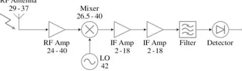
In this paper a PMMW imaging system, designed to detect objects in low-visibility conditions, is proposed for fitting under a UAV. PMMW images are formed by capturing the emissions from the target area using antennae and measuring the magnitude of the captured emissions with detectors. The simplest model is a single antenna operating at a single frequency directed at a single orientation scanned over the target area by a mechanical motor, as depicted in Fig 1.
Fig. 1. Total power peterodyne radiometer
The antenna captures the emissions, the mixer converts the radio frequency (RF) fRF signal to a lower intermediate frequency (IF) fIF signal using the local oscillator (LO) frequency fLO, the filter removes the unwanted mixing products and the detector converts the wanted signal to a power level, with the amplifiers strengthening the signal. Good noise performance is vital to deal with the emissions that are between 1010 and 107 times smaller than IR emissions.
The choice of atmospheric window is a compromise between price, transmission and resolution. Technology is immature within the transmission windows at 140GHz and 220GHz, thereby making these options not cost-effective. For a given antenna aperture the 94GHz window has greater spatial resolution, but the 35GHz window is chosen for the greater transmission through atmospheric constituents and thin layers of absorbent materials.
The speed of the simple model of Fig. 1 is increased by making use of multiple antennae, with the orientation of the antennae controlled using electronic, optical or mechanical techniques. The size of the UAV precludes any form of optical or mechanical scanning, thereby limiting the design to electronic scanning. In using the motion of the UAV to scan along the plane of the flight path, the antenna scans only along the plane perpendicular to the flight path.
Fig. 2. Antenna patterns at different frequencies
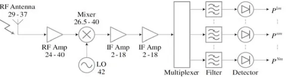
In using a frequency-scanned array for the antenna the captured emissions are split up into different frequency bands before detection to maintain the space-to-frequency mapping of the antenna. This is done by upgrading the simple model of Fig. 1 to include a multiplexer after the second IF amplifier and adding a filter and detector for each channel of the multiplexer, as depicted in Fig. 3.
Fig. 3. Multi-channel passive millimetre-wave imaging radiometer
The spatial resolution of an imaging system is defined by the number of resolvable pixels across the horizontal field of view, and is directly proportional to the size of the antenna and indirectly proportional to the wavelength of the emissions. MMW wavelengths are much longer than optical and IR wavelengths, requiring much larger antennae to achieve equivalent resolution to IR and optical imaging systems.
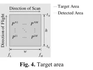
The image is built up line by line as the antenna concurrently scans the target area along the plane perpendicular to the flight path, with each orientation scanned by a beam at a different frequency f0m. The frequency range
L
f to fH is divided into M contiguous bands, each assigned to a different pixel column, Pm. The flight path time-period
0
t to tN is divided into
N measurements taken at discrete time-intervals, each assigned to a different pixel row, Pn.
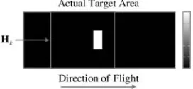
Fig. 4. Target area
When flying over the target area the image of an object is blurred along the plane of the flight path, making it difficult to determine the position of objects or to differentiate between objects situated along the plane of the flight path. Prevention is impossible as the size of the UAV precludes the use of bulky optics to focus the antenna along the plane of the flight path as well. The solution is a post-processor that reconstructs the target area from the blurred image.
3. Mathematical Model
Image degradation is conventionally defined in literature as a combination of blurring of the edges between regions and the addition of random noise to the image. The conventional methodology of image reconstruction is to invert the effect of the degradation. As blurring and noising have opposing effects, the reconstruction algorithm must balance deblurring and denoising to reconstruct the original image.
The conventional methodology makes use of algorithms incorporating iterative partial differential equations of the form zk1zk t zk /t, where t is the step size of the
algorithm and the reconstruction method is determined by the formulation of zk /t. There are three basic approaches to reconstruct an image, with the two denoising algorithm based on parabolic equations and the deblurring algorithm based on hyperbolic equations.
The canonical axiomatic approach to denoising is isotropic diffusion, which is equivalent to a smoothing process with a Gaussian kernel. Isotropic diffusion contains no mechanism to differentiate between regions in an image and diffuses the image as a whole. Anisotropic diffusion (Perona 1990) was introduced in order to locate and diffuse regions separately while maintaining sharp edges by constructing a nonlinear adaptive denoising process.
The canonical variational approach to denoising is total variation (Rudin 1992), which is a minimisation process. Total variation uses a globally defined scalar, , that results in fine detail being diffused. Adaptive total variation (Gilboa 2003) was introduced in order to preserve texture by locally reformulating . The locally defined results in each region being denoised separately to improve the detail retention during denoising.
The canonical approach to deblurring is the shock filter (Osher 1990), which behaves similar to deconvolution. The edges are sharpened by developing shocks at inflection points. The shock filter is sensitive to noise as noise adds inflection points to the image, disrupting the process and resulting in noise in the image being enhanced. The combination of diffusion and the shock filter was introduced in order to increase robustness to noise (Alvarez 1994).
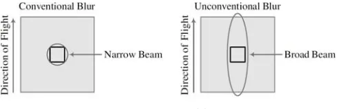
focused lens smoothes an image's edges between regions, as depicted in Fig. 5. Conventional blurring is localised as only the surrounding area is incorporated into the image.
Fig. 5. Image blur
In the proposed application the blurring problem is magnified as there is a many-to-one relationship between the target area and the detected signal due to the broad beam of the antenna. Each pixel of the image incorporates data from within the target area and outside of the target area, as depicted in Fig. 5. Conventional techniques cannot be used as they deal with localised object blurring, which is unable to counter the global object blurring of the antenna.
The Kalman filter is a set of mathematical equations that estimate a process by using feedback control. The time update equations projecting forward in time the current state estimate to the next time step and then the measurement update equations obtain feedback in the form of noisy measurements to adjust the projected estimate to obtain an improved estimate.
The non-stationary, discrete-time, linear process xk1n is modelled as
1
k k k k k k
x A x B u v (1)
where l k
u is the external control that drives the process from state xk to state xk1, vk is the process noise, n n matrix Ak relates state xk to state xk1 in the absence of both external
control uk and process noise vk and n l matrix Bk relates external control uk to state xk.
State xk is accessible from the noise contaminated measurement
m k
z modelled as
k k k k
z H x w (2)
where wk is the measurement noise and m n matrix Hk relates state xk to measurement zk.
Process noise vk and measurement noise wk are independent of each other, additive, zero-mean, white and Gaussian with normal probability distributions
( ~ ( , )
( ) ~ ( , ) )
k k
k k
p p
v 0 Q
w 0 R
(3)
where [ T]
k E k k
Q v v is the process noise covariance, [ T]
k E k k
R w w is the measurement noise covariance and [ T] 0 [ T],
k n k n
E v v Ew w n k .
A priori estimate 1| n kk
x of state xk1 is given by the expectation
1| [ 1| ]
k k k E k
where xi j| ,i j is the estimate of state xi using measurements { , , }0
j
j
Z z z up to and including time j and is obtained from the noise-free version of the process model of (1), a posteriori state estimate xk k| and external control uk.
A posteriori state estimate xk1|k1n is obtained from a priori state estimate xk1|k and the weighted difference between measurement zk1 and a priori measurement estimate zk1|k
1| 1 1| 1( 1 1| )
k k k k k k k k
x x K z z (5)
where n m matrix Kk1 is the Kalman gain. Kalman gain Kk1 is the optimal linear estimator
that minimises a posteriori error covariance Pk 1|k 1.
A priori state error covariance Pk1|k is obtained from a priori state estimate xk1|k
1| |
T k k k k k k k
P A P A Q (6)
where ek1|k xk1xk1|k is the a priori state estimation error.
A posteriori state error covariancePk 1|k 1is obtained from a posteriori state estimatexk 1|k 1
1| 1 1| 1| 1 1 1 1 1| 1( 1 1| 1 1) 1
T T T T
k k k k kk k k k k k k k k k k k k k
P P P H K K H P K H P H R K (7)
where ek 1|k 1xk1xk 1|k 1 is the a posteriori state estimation error.
Making the derivative of a posteriori error covariance Pk 1|k 1 with respect to Kalman gain
1
k
K equal to 0 and solving for Kk1 the optimal gain for a posteriori state estimate xk 1|k 1 is
1
1 1| 1( 1 1| 1 1)
T T
k k k k k k k k k
K P H H P H R (8)
which reduces a posteriori state error covariance Pk 1|k 1 of (7) to the well known form
1| 1 1| 1 1 1|
k k k k k k k k
P P K H P (9)
The recursion of a posteriori state error covariance Pk 1|k 1 of (9) is ill-conditioned
(Andrade-Cetto2005). As the filter converges, the cancelling of significant digits on a posteriori state error covariance Pk 1|k 1 leads to asymmetries or to a non positive semi definite (PSD) matrix, which
cannot be true from the definition of a posteriori state error covariance Pk 1|k 1. Therefore a
posteriori state error covariance Pk 1|k 1 of (9) is replaced by the Joseph form
1| 1 ( 1 1) 1| ( 1 1) 1 1 1
T
k k k k k k k
T
k k k k
P I K H P I K H K R K (10)
which is PSD given its quadratic nature.
For an uncertain measurement zk1 and precise a priori state estimate xk1|k the prediction of a posteriori state estimate xk 1|k 1 relies more on the process model of (1) than measurement
1
k
1|
1| 1 1|
1
1| 1 1|
lim k k
k k k k
k
k k k k
P 0 x x K 0
P P (11)
For a precise measurement zk1 and uncertain a priori state estimate xk1|k the prediction of a posteriori state estimate xk1|k1 relies more on measurement zk1 than the process model of (1)
and a posteriori state error covariance Pk1|k1 is considerably reduced
1
1
1| 1 1 1
1
1 1
1| 1
lim
k
k k k k
k k k k R 0
x H z
K H
P 0 (12)
The Kalman filter works because the combination of a priori state estimate xk1|k conditioned on measurements Zk and a posteriori state estimate
|
k k
x , with state xk distribution
| |
( k | k) ~ ( k k, k k)
px z x P (13)
into a posteriori state estimate xk1|k1 is an improved estimate of state xk1, based on the
probability principle that a more accurate estimate is obtained from the combination of two estimates, 2 1 2 1 2 1
1| 1 1| |
( k k ) ( k k) ( k k)
P P P .
4. Implementation
For the proposed application of airborne surveillance for search and rescue operations, the antenna is fitted under a UAV flying over the ocean. The target area is assumed to be a constant distance from the UAV and consist only of sea water at a uniform temperature. The only discrepancy from this continuum is the sea vessels being searched for. Reconstruction of the target area is required to determine the position of objects and to differentiate between objects.
For this proposal state xk is the target area, process evolution Ak models the change of the target area due to the flight of the UAV, measurement zk is the antenna output and measurement evolution Hk models the measured antenna pattern. The change from state xk to state xk1 is based entirely on the flight of the UAV, reducing the process model of (1) to
1
k k k k
x A x v (14)
There is a large overlap between the target area scanned by measurement zk and the target area scanned by measurement zk1, as depicted in Fig. 6. The extension to the front of the UAV seen
by measurement zk1 is predicted and the extension to the back of the UAV no longer seen by measurement zk1 is omitted, with the rest of the target area carried over from state zk.
As the target area is assumed to be static with a few slow moving objects on a stable background, the target area as seen by measurement zk is assumed to be equal to the target area as seen by measurement zk1. For the same reason the extension to the front on the UAV seen by measurement zk1 is predicted to be equivalent to the target area just before this extension.
Mathematically this is done by shifting pixel rows n| 2, , n N
P of a posteriori state estimate
|
k k
x unchanged into pixel rows n| 1, , 1 n N
P of a priori state estimate xk1|k and predicting pixel row PN of state
1
k
x as equal to pixel row PN of state
k
x using state evolution Ak defined as
' '
'
'
0 1 0 0
0 0 0
where
0 0 0 1 0 0 0 1 k k k k k
A 0 0 0
0 A 0 0
A A
0 0 0
0 0 0 A
(15)
A posteriori state estimate xk k| is initialised as xk k| |k00, a '
k
A is required for each pixel column Pm and pixel columns Pm of state
k
x are lexicographically ordered into one column for multiplication with state evolution Ak.
The antenna concurrently scans the target area along the plane perpendicular to the flight path, with each orientation scanned by a beam at a different frequency f0m. The frequency
range fL to fH is divided into M 9 contiguous bands, each assigned to a different pixel column, Pm. Even though the main beam at frequency
0m
f is orientated to a particular part of the target, the whole target area is measured at frequency f0m.
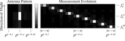
Therefore, the antenna patterns at the different frequencies f0m are combined to reconstruct the target area. Mathematically this is done by combining the M 9 measured 2D antenna patterns, Ant2D, into one measurement evolution Hk. Each row of measurement evolution Hk relates one frequency component of measurement zk to state xk, as depicted in Fig. 7.
Fig. 7. Measurement model
As the antenna has a narrow beam along the plane perpendicular to the flight path, only pixel column Pm is significant affected by
2D
Antm . As the antenna has a broad beam along the
plane of the flight path, many pixels within pixel column Pm are significant affected by
2D Antm .
This blurs the image, making it difficult to determine the position of objects or to differentiate between objects situated along the flight path.
| 0 1 2 0 3 0 T
k k k k k
T
kk k k
T
kk k k
P A A
Q A A
R H H
(16)
where1,2and3reflect the degree of uncertainty in the state, the measurement and the process.
Given the initial conditions of a posteriori state estimate xk k k| |0 and a posteriori state error
covariance Pk k k| |0, the Kalman filter is obtained iteratively by predicting the a priori estimates
1| |
1| 1|
1| |
k k k k k k k
k k k k k
T k k k k k k k
x A x B u
z H x
P A P A Q
(17)
and computing Kalman gain Kk1 to update the a posteriori estimates
1
1 1| 1 1 1| 1 1
1| 1 1| 1 1 1|
1| 1 1 1 1| 1 1 1 1 1
( )
( )
( ) ( )
T T
k k k k k k k k k
k k k k k k k k
T
k k k k k k k k k k
T k
K P H H P H R
x x K z z
P I K H P I K H K R K
(18)
5. Results
Specific target areas are simulated to test the ability of the Kalman filter to model the flight process and to remove the blur of the measurement process. The input parameters are gradually increased from idealised values to the expected values to simplify the optimisation process.
As a first experiment, the ability of the Kalman filter to model the flight process is tested for a target area containing a single frequency component and with measurement evolution Hk of size 9 27 based on antenna measurements using a reflector that concentrates antenna pattern Ant2D into a 1 1
main beam, as depicted in Fig. 8. This idealisation removes the
interfering effect of neighbouring frequency components and the blurring effect of the antenna pattern to simplify the problem to just one involving the modelling of the flight process.
Fig. 8. Idealised measurement model
Fig. 9. Idealised Single Frequency Target Area
For this position-velocity model pixel row PN of state 1
k
x is predicted as the sum of pixel row PN of state
k
x and the change between pixel row PN1 and pixel row PN of state
k
x and the change between pixel row PN1 and pixel row PN of state 1
k
x is equated with the change between pixel row PN1 and pixel row PN of state
k
x using state evolution Ak
'
'
'
'
0 1 0 0 0
0 0 0 0
where 0 0 0 1 0
0 0 0 1 1 0 0 0 0 1
k k
k k
k
A 0 0 0
0 A 0 0
A A
0 0 0
0 0 0 A
(19)
With no correlation between the velocity parameter xk of state xk and measurement zk, measurement evolution Hk of Fig. 8 is altered to a form of size 9 36 by inserting a zero-value column after each pixel column Pm, as depicted in Fig. 10.
Fig. 10. Idealised measurement model using position-velocity model
A second experiment is performed to test the ability of the Kalman filter to model the flight process for the same target area, but this time with measurement evolution Hk of size 9 108
based on antenna measurements using a reflector that concentrates antenna pattern Ant2D into a
1 10 main beam, as depicted in Fig. 11. The idealisation of the measurement model is
Fig. 11. Partially idealised measurement model
The response to the change between pixel row Pn and pixel row Pn1 of state k
x is spread over a number of pixels proportional to the width of the main beam, resulting in a blurred response in a posteriori state estimate xk k| to state xk, as depicted in Fig. 12. An improved response is obtained by increasing the number of time steps calculated per Kalman filter loop.
Fig. 12. Partially idealised single frequency target area
For this multi-measurement model state xk is extended by c pixel rows, where c is the number of extra time steps calculated per Kalman filter loop, which extends the size of each
'
k
A by c in state evolution Ak.
For this multi-measurement model the rows within measurement evolution Hk are repeated c times, but with a one pixel offsets due to the shift in focus from time step k to time step k1, as depicted for measurement evolution Hk of size 9 198 with c10 in Fig. 13.
Fig. 13. Partially idealised measurement model using multi-measurement model
The size of measurement evolution Hk has a direct effect on the number of time steps the Kalman filter takes to adapt to the model. The larger the area the main beam of antenna pattern
2D
Ant maps onto, the more pixels that need to be predicted concurrently in the initialisation of a posteriori state estimate xk k k| |0 and the longer the uncertainty period of a posteriori state
estimate xk k| . The uncertainty period for the 1 10
The reason for the improved response of the multi-measurement model is accredited to the increased size of measurement evolution Hk. For a single time step per Kalman filter loop and a single frequency component target area, the denominator of the Kalman gain Kk of (8) is a 1 1 matrix that can only globally rectify the Kalman gain Kk of size 12 1 , and thereby only globally rectify the pixels of state xk.
When the number of time steps is increased per Kalman filter loop to 11 with c10, the denominator of the Kalman gain Kk of (8) increases in size to 11 11 . In approaching the size of the Kalman gain Kk of 22 11 , the elements of Kalman gain Kk are rectified individually and thereby the pixels of state xk are rectified individually. Only when a large number of time steps are used per Kalman filter loop does 1
1
k k
K H when Rk10.
The final set of experiments test the ability of the Kalman filter to remove the errors in the measurement process using measurement evolution Hk of Fig. 13 and a full frequency range target area of size 9 50 containing a single central high intensity object of size 3 3
surrounded by a low intensity background, as depicted in Fig. 14. The last idealisation is removed to incorporate modelling of the interfering effect of neighbouring frequency components. The large size of measurement evolution Hk results in a long uncertainty period.
Fig. 14. Partially Idealised Full Target Area with Single Object
The variance in absolute gain between the M 9 components of antenna pattern Ant2D returns a false multi-level object and background, while the partial blurring of the object to neighbouring bands is accredited to non-ideal slope of the main beam. The Kalman filter is able to reduce both of these inaccuracies once the long uncertainty period has past, as depicted in Fig. 15.
Fig. 15. Predicted Target Area for Partially Idealised Full Target Area with Single Object
Fig. 16. Partially Idealised Full Target Area with Multiple Objects
The ability of the Kalman filter to reduce the variance in absolute gain between the M 9 components of antenna pattern Ant2D and the infringement of the main beam into neighbouring
bands is not affected by the number of objects within the target area. The blurring effect of antenna pattern Ant2D merges the closely spaced objects into a single object, with a false
higher intensity at the location of the two border objects. The Kalman filter is able to response quick enough to a change between pixel row Pn and pixel row Pn1 of state
k
x , resulting in the objects being individually sharpened and detached from each other, as depicted in Fig. 17.
Fig. 17. Predicted target area for partially idealised full target area with multiple objects
6. Conclusions
Advances in UAV technology have created the option of introducing PMMW imaging capability into an autonomous vehicle for low-visibility conditions. However, the size of the UAV places restrictions on the design of the system in the inability to incorporate any measure to focus the antenna pattern before image creation that leads to a non-ideal antenna pattern.
A technique is needed to reconstruct the image after image creation. Conventional image reconstruction processes deal with localised object blurring modelled by Gaussian noise, which is insufficient to counter the more global object blurring of the antenna pattern, and are designed for stationary stand-alone images.
This paper proposes a new unconventional technique based on the Kalman filter. For each time-interval the Kalman filter makes a prediction of the detected signal using the measured antenna pattern. The comparison between the predicted signal and the detected signal is used to generate an accurate image of the target area.
References
Alvarez L, Mazorra L (1994). Signal and Image Restoration Using Shock Filters and Anisotropic Diffusion, SIAM Journal on Numerical Analysis, 31(2), 590-605.
Andrade-Cetto, J (2005). The Kalman Filter, Tech Rep IRI-DT-02-01, Institut de Robótica i Informática Industrial, Universitat Politécnica de Catalunya, Barcelona, Spain.
Appleby R, Anderton RN (2007). Millimeter-Wave and Submillimeter-Wave Imaging for Security and Surveillance, Proceedings of the IEEE, 95(8), 1683-1690.
Chandrasekar V, Fukatsu H, Mubarak K (2003). Global Mapping of Attenuation at Ku- and Ka-Band, IEEE Transactions on Geoscience and Remote Sensing, 41(10), 2166-2176.
Gilboa G, Sochen N, Zeevi YY (2003). Texture Preserving Variational Denoising Using an Adaptive Fidelity Term, Proceedings of the VLSM, 137-144.
Hopper R (2005). System Solutions using MMW Sensors, Proceedings of ARMMS.
Kalman RE (1960). A New Approach to Linear Filtering and Prediction Problems, Transactions of the ASME - Journal of Basic Engineering, 82(Series D), 35-45.
Liebe HJ (1983). Atmospheric EHF Window Transparencies near 35, 90, 140, and 220 GHz, IEEE Transactions on Antennas and Propagation, 31(1), 127-135.
Osher S, Rudin LI (1990). Feature-Oriented Image Enhancement Using Shock Filters, SIAM Journal on Numerical Analysis, 27(4), 919-940.
Perona P, Malik J (1990). Scale-Space and Edge Detection Using Anisotropic Diffusion, IEEE Transactions on Pattern Analysis and Machine Intelligence, 12(7), 629-639.
Rudin LI, Osher S, Fatemi E (1992). Nonlinear Total Variation Based Noise Removal Algorithms, Physica D: Nonlinear Phenomena, 60, 259-268.
Ulaby FT, Moore RK, Fung AK (1986). Microwave Remote Sensing, 3, Artech House, USA. Wilson WJ, Howard RJ, Ibbot AC, Parks GS, Ricketts WB (1986). Millimeter-Wave Imaging