_____________________________________________________________________________________________________
International
23(2): 1-16, 2019; Article no.JGEESI.50722 ISSN: 2454-7352
The Use of Combined Geophysical Survey Methods
for Groundwater Investigation in a Typical Basement
Complex Terrain: Case Study of Erunmu, Ibadan,
Southwest Nigeria
Abudulawal, Lukuman
1*1Department of Geology, Faculty of Science, The Polytechnic, Ibadan, Oyo State, Nigeria.
Author’s contribution
The sole author designed, analysed, interpreted and prepared the manuscript.
Article Information
DOI: 10.9734/JGEESI/2019/v23i230165 Editor(s): (1) Dr. Iovine Giulio, CNR-IRPI (National Research Council – Institute of Research for the Geo-hydrologic Protection) of Cosenza, Italy. Reviewers: (1) Ibitoye Folahan Peter, Prototype Engineering Development Institute, Nigeria. (2)J. Dario Aristizabal-Ochoa, Universidad Nacional de Colombia, Colombia. (3)Matoh Dary Dogara, Kaduna State University, Nigeria. Complete Peer review History: http://www.sdiarticle3.com/review-history/50722
Received 20 June 2019 Accepted 27 August 2019 Published 10 September 2019
ABSTRACT
A combined Survey involving the very low frequency electromagnetic (VLF – EM) and Electrical resistivity surveys were carried out in order to appraise the groundwater potential, and locate appropriate positions for sighting boreholes in Erunmu Community, Egbeda local government area, Oyo State, Nigeria. VLF data were obtained along five traverses as the first step in order to locate suitable vertical electrical sounding (VES) stations. Vertical Electrical Soundings using Schlumberger array were thereafter carried out at twenty 20) locations. The integrated interpretation of both data confirms the presence of aquifers, which includes, weathered zone and basement transition/fractures beneath the area, which prior to this investigation have a history of failed boreholes and wells. The resistivity curve types obtained includes H and A which revealed the presence of 3 to 4 subsurface layers consisting of topsoil, the clay, the sandy clay, fractured zone and the highly resistive bedrock. The resulting geo-electric section from the interpretation revealed the Reflection coefficient which ranges from 0.45 – 0.98. The dominated curve type in the area investigated is the H which is typical of basement complex while the A-type is about 20% of the total curves. Hydrogeological, the topsoil is not important because the degree of water
saturation in this layer is very low and cannot be utilized for groundwater. The fractured basement layer (which is present in less than 15% of the study area is very relevant in groundwater prospecting; when it is thick enough the layer could support borehole drilling. Areas identified as geological interfaces in the VLF anomaly charts were also confirmed by the interpreted VES data as poor and intermediate zones for groundwater potential in the study area. The significance of this study is such that it will serve as a useful reference for future research efforts in the aspect of basement complex groundwater studies.
Keywords: Vertical electrical sounding (VES); VLF-EM; reflection coefficient; basement layer.
1. INTRODUCTION
Groundwater occurrences in Precambrian basement terrain are hosted within zones of weathering and fracturing which often are not continuous in vertical and lateral extent. Electromagnetic (EM) profiling and VES are the two complementary and widely used geophysical methods in the delineation of basement regolith and location of fissured media and associated zones of deep weathering in crystalline terrains. In many instances, reconnaissance EM surveys are used to locate aquiferous zones such as fractures, faults and joints while Vertical Electrical Sounding, on the other hand, provides information on the vertical variation in electrical resistivity with depth. It is commonly used to assess the reliability of the fractures delineated from the EM survey [1,2]. Electrical resistivity (ER) and very-low-frequency electromagnetic induction (VLF) surveys are sensitive to groundwater quality medium [3,4,5,6,7,8,9]. The electromagnetic (EM) VLF methods have found a useful application in site investigation for groundwater development, most especially in
basementcomplexareas[10,11,12].Its relevance
is claimed to be in overburden thickness (Depth to basement bedrock) estimation and basement fracture delineation [13].
The electrical resistivity method is a unique geophysical tool used in groundwater and landfill studies [14,15]. The resistivity method is used for electrical sounding and imaging. The electrical sounding provides information about vertical changes in subsurface electrical properties and thus, it is useful in the determination of hydrogeologic conditions such as the depth to the water table, depth to bedrock, and thickness of soil [14,16].
2. MATERIALS AND METHODS
2.1 The Study Area
The study area is located at Erunmu, Nigeria which is demarcated by the following coordinates
latitude 70 25‘ N to 70 27’ N and longitude 40 3’ E
to 40 4’ E, within the humid tropical region with
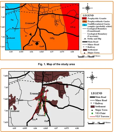
two distinct seasons. The rainy season could be demarked from March to October and dry season from November to March. The basement complex is divided into two provinces. The Western Province and the Eastern province. The Western Province has comprised of NNE-SSW trending schist belts separated from one another by migmatites, gneisses and granites and the Eastern Province comprises mainly migmatites, gneisses and large masses of Pan-African granitoid (Older Granites) intruded in Jos plateau, by Jurassic peralkaline granites as shown in Figs. 1 and 2.
2.2 Method of Data Acquisition
The geophysical investigation involved the Very Low Frequency (VLF) Electromagnetic and
Electrical Resistivity methods. These two
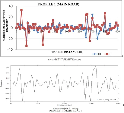
methods are both responsive to water-bearing fractures columns due to their relatively high-bulk electrical conductivities. The Electrical Resistivity method involved the vertical electrical sounding (VES) with the use of the Schlumberger array. The soundings (twenty in all) were carried out at locations of prominent VLF anomalies, which are presumably typical of basement fractures. The VLF-EM measurements were made at 5.0m interval along with five (5) approximately
North-South Traverses (Fig. 2). The VLF Traverses
range in length from 150- 600m. The ABEM WADI VLF-EM meter was used for the data collection. The equipment measured the real
(in-phase) and quadrature (out of phase)
components of the vertical to horizontal magnetic field ratio.
in-phase). The data collected along the existing routes were filtered using both Fraser and Karous-Hjelt filters, thereby providing a means of removing geologic and noise originating from the transmitter. Karous and Hjelt [17] filter computes approximate current density of the subsurface giving rise to relative data across the resulting profiles [18]. In a similar way, the Fraser filter transforms the VLF anomalies to contours in such a way that proper crossovers are transformed to positive peak readings, while reverse crossovers become negative values [8]. The VLF survey was carried out by collecting
data along five (5) trasverses and modeling this using computer software (KHFIT), from which twenty (20) VES stations were delineated in the study area. The data collected from the twenty (20) stations were interpreted manually using partial curve matching to obtain the initial model parameters, while these parameters were fed into the computer using a specialized software (RESIST 1.0) in order to obtain the final model
parameters, which were then analyzed
qualitatively using type curves and geo-electric
section to evaluate the sub-surface
hydrogeological conditions.
Fig. 1. Map of the study area
3. RESULTS AND DISCUSSION
Qualitative and semi-quantitative interpretations of the VLF-measurements profiles were made to map occurrence of localized alterations of conductive and resistive rocks as well as
contacts among materials of different
conductivity. Figs. 3-7 shows typical inverted current density pseudo sections and smoothened real components obtained using the Karous-Hjelt’ 2D-inversion program named KHFfilt Version 1.1a. The pseudo sections are displayed as the equivalent current density estimated from the filtered real component of the VLF data. The colour pane indicates a bluish to green colour for the resistive medium, while yellowish to red colour range indicates conductive medium. The locations of the conductors are specified by cross over points in the in-phase and a positive peak in the filtered-real (current density) plots as shown in Figs. 3a, 4b, 5c, 6d and 7e, while location and identification of proper cross over points are enhanced in the Fraser filtered data in Figs. 3-7.
The Fraser filtered data improves identification of the conductive anomalies and removes false impression from the false cross-over points that usually make interpretation of the measured data difficult.
Along profile 1, the current density profile shows existence of two anomalies located at 30m and 340m. A shift in the location of the two anomalies is indicated in the in-phase component plot. The first anomaly has the appearance of an anomaly over a conductive zone with southward orientation and is shallower in depth. The corresponding filtered real using Fraser filter helps to delineate the location of these anomalies as well as collapsing the false cross over points that usually makes interpretation of the measured data difficult. Series of shallow and near surface bodies, which were recognized as conductive bodies on the pseudo -section (Fig. 2): have low amplitude.
VLF results tend to be rather noisy, being distorted by minor anomalies due to small local (usually artificial) conductors and electrical interference. Noise can be reduced by adding together results recorded at closely spaced stations and plotting the sum at the mid-point of the station group. This is the simplest form of low-pass filter.Two common types of filtering designed to carry out these operations are; The
Fraser filteruses four equal-spaced consecutive
readings. The first two are added together and halved. The same is done with the second two and the second average is then subtracted from the first. The more complicated Karous–Hjelt filter utilizes six readings, three on either side of
a central reading that is not itself used. The ABEM WADI instrument automatically displays K–H filtered data unless ordered not to
do so.
The interpretation of WADI data is generally based on the filtered real part with the aid of the Karous-Hjelt filter, which enables the distribution of the current density responsible for the secondary magnetic field to be displayed as the isovalue maps and interpreted as maps of current density [18]. The filter therefore provides a pictorial indication of the depth of the various current concentrations and hence the spatial dispositions of subsurface geological features, such as mineral veins, faults, shear zones and stratigraphic conductors [19]. Filtered data used to contour the K–H filter can also be used to
compute current-density pseudo-sections.
Information on the nature of overburden can be deduced from the filtered imaginary part. However, VLF data cannot be used to determine patterns of simultaneous current flow at different depths.
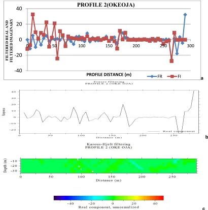
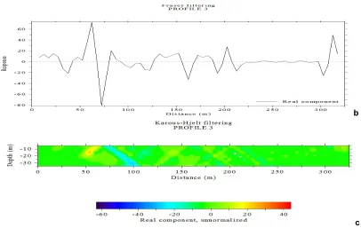
Along profile 2, there is no anomaly observed on the pseudo-section displayed (Fig. 4). The Fraser filter shows that the real component has no peak along the profile line. There are no conductive zones along the profile. The graph plotted on the excel show that there is no positive peaks for the profile and it shows that the place is highly resistive. Profile 3, with (Fig. 5) Showing a single anomaly which is seen at 73 m along the profile line on the plotted graph, on the Fraser filter plot and on the pseudo-section. The characteristic amplitude of these anomaly revealed that the conductors are relatively nearer to the surface and is at the point where it was identified i.e. it does not spread.
a
b
c
Fig. 3. The graph of the Filtered Real and Filtered Imaginary, smoothed in-phase Fraser filter and Inverted 2-D pseudo sections of the VLF-EM real component data for the profile 1
Profile 5, with E-W orientation shows
characteristic anomalies indicating a source in Fig. 7, which was later recognized as extensive on the pseudo-section at a deeper depth which is encountered at between 75 and 105 m. The anomalies were also identified with similar
signature the characteristic amplitude of these anomalies revealed that the conductors are relatively at a deeper depth. The pseudo current
density section also revealed a deeper
conductive zone.
-40
-20
0
20
40
0 50 100 150 200 250 300 350 400
FI
LT
ER
ED
R
EA
L
A
N
D
F
IL
TE
R
ED
IM
A
G
IN
A
R
Y
PROFILE DISTANCE (m)
PROFILE 1 (MAIN ROAD)
a
b
c
Fig. 4. The graph of the filtered real and filtered imaginary smoothed in-phase fraser filter and Inverted 2-D pseudo sections of the VLF-EM real component data for the profile 2
a
-40
-20
0
20
40
0 50 100 150 200 250 300
F
IL
T
E
R
E
D
R
E
A
L
A
N
D
F
IL
T
E
R
E
D
I
M
A
G
IN
A
R
Y
PROFILE DISTANCE (m)
PROFILE 2(OKEOJA)
FR FI
-40 -20 0 20 40 60
0 50 100 150 200 250 300
FI
LT
ER
ED
R
EA
L
A
N
D
F
IL
TE
R
ED
IM
A
G
IN
A
R
Y
PROFILE DISTANCE (m)
PROFILE 3
b
c
Fig. 5. The graph of the Filtered Real and Filtered Imaginary, smoothed in-phase Fraser filter and Inverted 2-D pseudo sections of the VLF-EM real component data for the profile 3
a
b
-40
-20
0
20
40
0 100 200 300 400 500 600
FI
LT
ER
E
D
R
EA
L
A
N
D
F
IL
TE
R
ED
IM
A
G
IN
A
R
Y
PROFILE DISTANCE (m)
PROFILE 4 (MAIN ROAD 2)
c
Fig. 6. The graph of the Filtered Real and Filtered Imaginary, smoothed in-phase Fraser filter and Inverted 2-D pseudo sections of the VLF-EM real component data for the profile 4
a
b
c
Fig. 7. The graph of the Filtered Real and Filtered Imaginary, smoothed in-phase Fraser filter and Inverted 2-D pseudo sections of the VLF-EM real component data for the profile 5
-40
-20
0
20
40
0
20
40
60
80
100
120
140
FI
LT
ER
ED
R
EA
L
A
N
D
FI
LT
ER
ED
IM
A
G
IN
A
R
Y
PROFILE DISTANCE (m)
PROFILE 5 (ORE KEKE)
3.1 Iso-value Maps of the Real
Fig. 8 presents the outputs of the filtered real component data as maps of the Fraser-filtered in-phase and equivalent Karous-Hjelt filtered (current density) maps. The maps clearly show the rock types in the area as indicated by various
zones with varying conductivity contrast.
Although, it is difficult to differentiate the rocks based on the observed anomalies, however, the identification of location and lateral extent of these rock types can be easily realized from these maps. The current density map showed that the conductive zone in the area can be found in the southwestern part of the map. The map clearly showed that the porphyroblastic gneiss that underlain the area investigated do not have conductive zones within it and this means that weathering of the basement is not deep. The southwestern part of the map may be considered for groundwater development in that area because of the conductivity of the rock in the area. The 3-D map of the isovalues of the current density gives the disposition of the conductivity of the area investigated and it show that the area is resistive and there is little or no conductive zone in the area. Electrical resistivity method was used by [20] for groundwater investigation in parts of
the Basement terrain in Southwest Nigeria and concluded also, that the weathered layer and the fractured Basement constitute the aquifer zones.
Very low frequency electromagnetic and vertical electrical sounding techniques was used by [21] in delineating aquifer zones in Modakeke area, Ife, Osun State. Electrical resistivity method was used by [22] in investigation of geo-electric and hydro-geologic characteristics of areas in Southwest Nigeria. Electromagnetic surveys by VLF-WADI Resistivity sounding was used by [23]
to interpret the geologic structures and
groundwater movement through fractures rock.
The manual interpretation and computer iteration of the VES data produced the dominated curve type in the area investigated is the H which is typical of basement complex while the A type is about 20% of the total curves. Hydro-geologically, the topsoil is not important because the degree of water saturation in this layer is very low and cannot be utilized for groundwater. The fractured basement layer which is present in less than 15% of the study area is very relevant in groundwater prospecting when it is thick enough the layer could support borehole drilling.
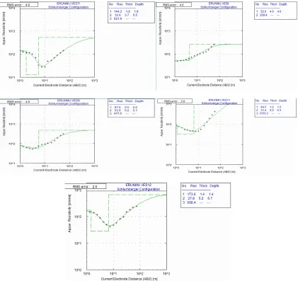
3.2 Vertical Electrical Sounding (VES) Curves
The VES curve types is predominantly the H-type and some A-type which typified basement terrain. The H-type show a system of three geo-electric layers of the topsoil, weathered basement and fractured/fresh basement while the A-type showed two geo-electric layers of the topsoil and the fresh basement. The figures presented below show the interpreted curves that were generated after curve matching and computer iteration using Resist 1.1 version.
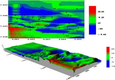
3.3 Isopach Map of the Overburden
Fig. 12 shows the overburden thickness for the surveyed area. The overburden as used in this work includes all materials above the presumably fresh bedrock. The map shows overburden thickness ranging between 2 and 13.4 m. The overburden is relatively not too thick around the
southern part 10–13.4 m and the overburden in the central and the far north eastern part is very shallow while the overburden generally in other area is shallow [16].
Generally, the overburden of the study area is dominantly shallow when compared to the range given by [24] and [25]. The groundwater abstraction from the weathered or fractured basement may not be too feasible because of the occurrence of shallow overburden and the little or no existence of fractured zone in the investigated area.
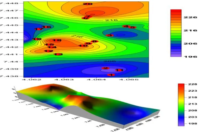
3.4 Bedrock Relief Map
Fig. 13 shows the contour map of the bedrock elevation for the VES points. This bedrock relief map shows the basement topography, its structural resolution and also the degree of weathering of the basement. The hydrogeologic importance of this has been identified by [24].
11
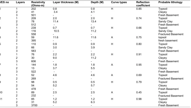
Table 1. Interpreted resistivity result for vertical electrical sounding VES
VES no Layers Resistivity (Ohms-m)
Layer thickness (M) Depth (M) Curve types Reflection coefficient
Probable lithology
1 1 202 0.8 0.8 H 0.85 Topsoil
Clayey
Fresh Basement
2 41 3.4 4.1
3 501 - -
2 1 209 2.0 2.0 H 0.74 Topsoil
Sandy Clay Fresh Basement
2 78 11.4 13.4
3 512 - -
3 1 239 0.7 0.7 H 0.66 Topsoil
Sandy Clay
Fractured Basement
2 116 10.5 11.2
3 558 - -
4 1 59 11.6 11.6 A 0.75 topsoil
fresh basement
2 395 - -
5 1 110 0.9 0.9 H 0.80 Topsoil
Sandy Clay Fresh Basement
2 66 3.0 3.9
3 583 - -
6 1 76 2.2 2.2 H 0.91 Topsoil
Clayey
Fresh Basement
2 30 9.0 11.2
3 606 - -
7 1 144 1.8 1.8 A 0.95 Topsoil
Clayey
Fresh Basement
2 13 3.7 5.5
3 522 - -
8 1 52 4.6 4.6 A 0.69 Topsoil
Fractured Basement
2 269 - -
9 1 98 0.5 0.5 H 0.79 Topsoil
Clayey
Fresh Basement
2 54 5.2 5.7
3 478 - -
10 1 89 2.5 2.5 A 0.45 Topsoil
Fractured Basement
2 232 - -
11 1 85 1.2 1.2 H 0.98 Topsoil
Clayey
Fresh Basement
2 31 5.2 6.3
12
VES no Layers Resistivity (Ohms-m)
Layer thickness (M) Depth (M) Curve types Reflection coefficient
Probable lithology
12 1 173 1.4 1.4 H 0.92 Topsoil
Clayey
Fresh Basement
2 28 5.2 6.7
3 668 - -
13 1 136 1.1 1.1 H 0.64 Topsoil
Sandy Clay
Fractured Basement
2 76 10.3 11.4
3 355 - -
14 1 301 1.2 1.2 H 0.84 Topsoil
Clayey
Fresh Basement
2 54 5.6 6.8
3 601 - -
15 1 211 1.3 1.3 H 0.98 Topsoil
Clayey
Fresh Basement
2 18 2.7 4.0
3 1662 - -
16 1 166 1.0 1.0 H 0.88 Topsoil
Clayey
Fresh Basement
2 55 4.8 5.8
3 858 - -
17 1 72 1.2 1.2 H 0.64 Topsoil
Sandy Clay
Fractured Basement
2 66 7.3 8.5
3 305 --
18 1 158 1.5 1.5 H 0.97 Topsoil
Clayey
Fresh Basement
2 19 2.8 4.3
3 1409 - -
19 1 224 2.6 2.6 H 0.91 Topsoil
Clayey
Fresh Basement 2
3
33 783
8.5 -
11.1 -
H
20 1 156 1.2 1.2 H 0.96 Topsoil
Clayey
Fresh Basement
2 40.5 4.8 6.0
3 2103.7 - -
Fig. 10. The Layer model interpretation for VES 7, 8, 9, 11 and 12
Fig. 12. The contour and the 3-D map of the overburden thickness of the area investigated
Topographic depressions and ridges are
identified in the bedrock relief map. The depressions are characterized by the thick overburden as seen in the southern part of the map while ridges are noted for thin overburden cover as seen in the central and the northern part
of the map. In addition to been characterized by thick overburden, basement depressions also
constitute groundwater collecting troughs,
especially the water displaced from the bedrock crest.
4. CONCLUSIONS
Based on the electrical resistivity survey conducted in the study area, groundwater potential producing zones have been delineated. The study reveals that about 90% of the study area has poor groundwater potential.The major drive was the fact that the area has a history of failed wells and boreholes due to lack of pre-drilling geophysical survey, thus resulting in shortage of potable water. Therefore, this effort aims at using geophysics to delineate part of the
basement where sustainable amount of
groundwater can be found. This was done using VLF – EM and electrical resistivity (VES) methods of survey.
ACKNOWLEDGEMENT
The author would like to appreciate my 2013/2014 project students and Mr. Afolabi during data acquisition.
COMPETING INTERESTS
Author has declared that no competing interests exist.
REFERENCES
1. Ariyo SO, Adeyemi GO, Oyebamiji AO.
Electromagnetic VLF survey for
groundwater development in a contact terrain: A case study of Ishara-Remo, Southwestern Nigeria. Journal of Applied Science Research. 2009;5(9):1239-1246.
2. Olayinka AI, Amidu SA, Oladunjoye MA.
Use of electromagnetic profiling and sounding for groundwater exploration in the crystalline basement area of Igbeti, Southwestern Nigeria. Global Journal of Geological Science. 2004;2(2):243-253.
3. Kelly EW. Geoelectric sounding for
delineating ground water contamination. Ground Water. 1976;14:6-11.
4. Koefoed O. Resistivity sounding on an
Earth model containing Transition Layers with Linear change of Resistivity with Depth Geophysical Prospecting. 1979b;27: 862-868.
5. Urish DW. The practical application of
surface electrical resistivity to detection of groundwater pollution: Ground Water. 1983;21:144–152.
6. Mazac O, Kelly WE, Landa I. Surface
geo-electrics for groundwater pollution and
protection studies. J. Hydro. 1987;93:277-294.
7. McNeill JD. Use of electromagnetic
methods for groundwater studies,
in Ward, S. H., Ed., Geotechnical and
environmental geophysics. Soc. of Expl. Geophys. 1990;1:191–218.
8. Telford WM, Geldart LP, Sheriff RA.
Applied geophysics, 2nd edition: Cambridge
Univ. Press; 1990.
9. Burger HR. Exploration geophysics of the
shallow subsurface: Prentice-Hall, Inc.; 1992.
10. Olorunfemi MO, Afolayan JF, Afolabi O.
Geoelectric/Electromagnetic VLF Survey for groundwater in a basement terrain: A case study. Ife Journal of Science. 2004; 6(1):74-78.
11. Olayinka AI. Electromagnetic profiling and
resistivity soundings in groundwater
investigation near Egbeda, Kabba, Kwara State. Journal of Mining and Geology. 1999;27(2):243-250.
12. Omosuyi GO, Adeyemo A, Adegoke AO.
Investigation of groundwater prospect using electromagnetic and geoelectric sounding at Afunbiowu, near Akure, Southwestern Nigeria. Pacific Journal of Science and Technology. 2007;8(2):172-182.
13. Sundrarajan N, Nandakumar G.
Narsimhachary M, Ramam K, Srinivas Y.
VES and VLF—an application to
groundwater exploration, Khammam,
India., The Leading Edge. 2007;708-716.
14. Zohdy AAR. Earth resistivity and seismic
refraction investigation in Clara County,
California, PhD thesis (unpublished).
Stanford University. 1964;131-135.
15. Dahlin T, Zhou B. Gradient and midpoint
referred measurements for multichannel
2D resistivity imaging. Proc. 8th meeting of
the environmental and engineering
geophysics. Aveiro, Portugal; 8-12
September. 2002;157-160.
16. Abudulawal L, Amidu, Sakiru A, Apanpa
KA, Adeagbo OA, Akinbiyi OA.
Geophysical investigation of subsurface water of Erunmu and its environs,
Southwest Nigeria using electrical
resistivity methods. Journal of Applied Sciences. 2015;15(5):741-751.
17. Karous M, Hjelt SE. Linear filtering of VLF
dip-angle measurements: Geophysical
Prospecting. 1983;31:782-794.
18. Benson AK, Payne KL, Stubben MA.
DC resistivity and VLF geophysical methods - a case study. Geophysics. 1997;62:80-86.
19. Ogilvy RD, Lee AC. Interpretation of
VLF-EM in phase data using current density pseudosections. Geophysical Prospecting. 1991;39:567-580.
20. Olorunfemi MO, Mesida EA. Engineering
Geophysics and its application engineering site investigations (case study from Ile-Ife area). The Nigerian Engineer. 1987;22(2): 57-66.
21. Osuagwu BC. Geophysical investigation
for groundwater in a difficult terrain around
Modomo Area, Ife, Osun State:
Unpublished Bachelor of Science Thesis, Obafemi Awolowo University, Ile-Ife, Osun State. 2009;88.
22. Olorunfemi MO, Fasuyi SA. Aquifer types
and Geoelectrical / hydrogeologic
Characteristics of Central Basement
Terrain of Nigeria. Journal of African Earth Science. 1993;16:309-317.
23. Sharma SP, Baranwal VC. Delineation of
groundwater – bearing fractured zones in a hard rock area integrating Very Low Frequency Electromagnetic and Electrical
Resistivity data. Journal of Applied
Geophysics. 2005;57:155–166.
24. Dan-Hassan MA, Olorunfemi MO.
Hydro-geophysical investigation of a
basement terrain in the North-Central part of Kaduna State, Nigeria. Journal of Mining and Geology. 1999;12:189-206.
25. Omosuyi GO, Ojo JS, Enikanselu PA.
Geophysical investigation for groundwater around Obanla – Obakekere in Akure Area
within the basement complex of
southwestern Nigeria. Journal of Mining and Geology. 2003;39(2):109–116. _________________________________________________________________________________
© 2019 Lukuman; This is an Open Access article distributed under the terms of the Creative Commons Attribution License (http://creativecommons.org/licenses/by/4.0), which permits unrestricted use, distribution, and reproduction in any medium, provided the original work is properly cited.
Peer-review history: