Nelson

Forestry & Natural-Resource Sciences Last Correction: Aug. 2, 2011

CONSISTENCY OF FOREST PRESENCE AND BIOMASS

PREDICTIONS MODELED ACROSS OVERLAPPING SPATIAL

AND TEMPORAL EXTENTS

M. D. Nelson

, S. P. Healey

, W. K. Moser

, J. G. Masek

, W. B. Cohen

1_{U.S. Forest Service Northern Research Station, 1992 Folwell Avenue, St. Paul, MN, 55108, USA} 2_{U.S. Forest Service Rocky Mountain Research Station, 507 25th Street, Ogden, UT, 84401, USA} 3_{Goddard Space Flight Center, National Aeronautics and Space Administration, Greenbelt, MD, 20771, USA} 4_{U.S. Forest Service Pacific Northwest Research Station, 3200 SW Jefferson Way, Corvallis, OR 97331, USA}

Abstract._{We assessed the consistency across space and time of spatially explicit models of forest presence}

and biomass in southern Missouri, USA, for adjacent, partially overlapping satellite image Path/Rows, and for coincident satellite images from the same Path/Row acquired in different years. Such consistency in satellite image-based classification and estimation is critical to national and continental monitoring programs that depend upon processed satellite imagery, such as the North American Forest Dynamics Program. We tested the interchangeability of particular image acquisitions across time and space in the context of modeling forest biomass and forest presence with a non-parametric Random Forests-based approach. Validation at independent USA national forest inventory plots suggested statistically consistent model accuracy, even when the images used to apply the models were acquired in different years or in differ-ent image frames from the images used to build the models. For mapping projects using near-anniversary date imagery and employing careful radiometric correction, advantages of image interchangeability include the ability to build models with more ground data by combining adjacent image frames and the ability to apply models of assessed accuracy to early satellite images for which no corresponding field data may be available.

Keywords: Consistency analyses, North American Forest Dynamics, NAFD, Landsat, Random Forests, forest inventory, FIA.

1

Introduction

1.1 Modeling framework When field

measure-ments of forest attributes are combined in a modeling or classification framework with synoptic, remotely sensed data to produce spatial products, a fundamental as-sumption is made. Specifically, it is assumed that the nu-meric relationship between the forest attribute and the remotely sensed data, as observed at the locations for which field data are available, remains stable across the spatial field over which the attribute is being mapped, provided the inventory plots represent the forest condi-tions of interest contained within said image in an un-biased manner. At the simplest level, one assumes that a model based on forest inventory plots and a corre-sponding satellite image may be applied to all the image pixels not sampled by the plots. In this case, care must be taken only to assure that any anomalies (e.g. clouds,

sensor errors) in the remote image are identified and either corrected or excluded. However, when a model-ing framework calls for the combination of images from multiple acquisitions, each with their own radiometric and associated vegetation phenological properties, it be-comes necessary to standardize the interpretation of re-motely sensed values. In this case, all imagery must either be theoretically corrected to some standard ab-solute scale such as surface reflectance, or the imagery must be empirically cross-calibrated in some way, often using correction factors developed at invariant features where the images overlap. All discussions here will focus on satellite-derived optical reflectance data from passive sensors.

While multiple mapping projects have modeled for-est characteristics across large areas using many satel-lite image frames (e.g., Blackard et al., 2008, Hme et

al., 2001, Hansen et al., 2003, Kennedy & Bertolo, 2002, Pivinen et al., 2003, Ruefenacht et al., 2008), there is growing impetus to extend models not only over space but also over time (Woodcock et al., 2001). Time series of satellite imagery have the potential to yield uniquely consistent and exhaustive forest change data, particu-larly if data are acquired from a long-serving platform such as Landsat that has spatial and spectral properties adequate for detecting forest change (Cohen & Goward, 2004).

The North American Forest Dynamics Project (NAFD; see Goward et al., 2008) has initiated work across the USA to apply models of forest biomass to a 25-year (1985-2009) time series of radiometrically cor-rected Landsat imagery. These models are being cal-ibrated with recent field inventory measurements from the U.S. Forest Service Forest Inventory and Analysis Program (FIA), which is the national forest inventory of the USA. NAFD models are applied to time series of satellite imagery, including dates that precede field in-ventory data acquisition. The primary goal of NAFD is to describe the effects of disturbance and re-growth on forest carbon stores. A similar approach was taken by Healey et al. (2006) to identify forest canopy dis-turbance in the Pacific Northwest region of the USA. Healey et al. (2006) developed a change detection strat-egy, called “State Model Differencing,” in which mapped pre- and post-disturbance estimates of basal area and percent canopy cover estimates were used to label dis-turbance magnitude in concrete biophysical terms. This alignment of spectral change signals with traditional est metrics may in some cases be more useful for for-est managers than simple classifications of greater- and lesser-severity events (e.g., Kirschbaum, 2008, Nelsonet al., 2009). Powell et al. (2010) examined the accuracy of NAFD’s time series maps of forest biomass by using field measurements from multiple points in time. There are also pixel-level temporal smoothing techniques that may be applied to time series of forest condition maps to further reduce year-to-year variation caused by either random error or remaining calibration errors (Powellet al., 2010).

This study was designed to assess whether models of both aboveground standing biomass and forest/non-forest (f/nf) condition would yield predictions of com-parable accuracy if the satellite inputs for those models were acquired either in a different place or in a differ-ent year than the satellite data used to construct the models originally. While it would be impossible to as-sess the effects of every possible image artefact on the transferability of forest models from one image frame to another or from one date to the next, the goal of this study was to evaluate the degree to which model ac-curacy is affected when carefully chosen and calibrated,

near anniversary date imagery is used interchangeably in a modeling project. Application of models across time and space is interpreted as having no impact on model accuracy if statistical tests of model outputs using inde-pendent field observations produce non-significant differ-ences atα=0.05. The objective of this study is to con-duct an explicit assessment of the assumed image cross-calibration when the forest modeling frame requires that spectral relationships and models derived from one im-age be applied to imim-ages either from other times or other locations.

Results from this evaluation should be of use to NAFD and other projects that are combining archives of Land-sat or similar imagery with forest inventory data across large areas and long time periods.

1.2 Random Forests Ensemble approaches to clas-sification and estimation are becoming increasingly pop-ular because ensemble models are often more accurate than individual models (Opitz & Maclin, 1999). Im-proved classification accuracy is sought by aggregating the classifications of a diverse set of classifiers (Steele, 2000, Zhu, 2010). Ensemble aggregations are obtained by “stacking” multiple predictions, often involving re-sampling of the training dataset (Behrens et al., 2009). Breiman (1996b) described “stacked regressions”, fol-lowing the idea of stacking in Wolpert (1992). LeBlanc and Tibshirani (1996) suggest that the approach of stacked regressions is identical to the “model-mix” ap-proach proposed earlier by Stone (1974). Chan and Paelinckx (2008) describe ensemble classifications as falling into one of two general categories: 1) those based on a single learning algorithm, but with multiple varia-tions of the training set, and 2) those based on a combi-nation of several different learning algorithms, but with the same training set.

Random Forests (RF; Breiman, 2001), also known as “Breiman Cutler classifications” (BCC; Lawrence et al., 2006) falls within the first ensemble category. RF is a non-linear and non-parametric approach that can address complex multivariate interactions of predictors (Strobl et al., 2008, Strobl et al., 2007). In multi-dimensional data, RF characterizes and exploits struc-ture for the purposes of classification and prediction (Cutler et al., 2007). By permutation of independent variables, RF provides local and global measures of vari-able importance (Evans & Cushman, 2009).

achieved using the same imagery with a support vec-tor machine classifier (SVM; Vapnik, 2000), but the RF classifier had several operational benefits over the SVM classifier. Using RF with Landsat satellite imagery and ancillary datasets, Prasad et al. (2006) reported kappa coefficients of 0.60 to 0.68 for classifications of four in-dividual tree species in the eastern USA, and Gislason et al. (2006) reported classification accuracies ranging from 28 to 99 percent for nine forest types within Col-orado, USA. Gislason et al. (2006) compared the ac-curacy of RF with other ensemble classifiers, all using Landsat Multispectral Scanner (MSS) satellite remote sensing imagery and geographic data from a mountain-ous area of Colorado, USA. In terms of accuracies, RF outperformed a single Classification and Regression Tree (CART) classifier and was comparable to accuracies ob-tained by other ensemble methods (bagging and boost-ing). Furthermore, RF was much faster than the other ensemble methods, did not overfit, and could be used to estimate the importance of variables and detect outliers. Cutler et al. (2007) described applications of RF clas-sifier for three ecological presence-absence classifications, including invasive plant species presence in Lava Beds National Monument, California, USA, rare lichen species presence in the Pacific Northwest, USA, and nest sites for cavity nesting birds in the Uinta Mountains, Utah, USA. Five measures of classification accuracies result-ing from the RF classifier were compared with those of four other classifiers: linear discriminant analysis, logis-tic regression, additive logislogis-tic regression, and classifica-tion trees. For all three presence-absence applicaclassifica-tions, RF classifications were reported as being moderately to highly superior to the alternate methods tested. Cut-ler et al. (2007) summarized beneficial characteristics of RF as including, “(1) very high classification accuracy; (??) a novel method of determining variable importance; (??) ability to model complex interactions among pre-dictor variables; (??) flexibility to perform several types of statistical data analysis, including regression, classifi-cation, survival analysis, and unsupervised learning; and (??) an algorithm for imputing missing values.”

1.2.2 RF Estimation Hudak et al. (2008) compared estimates of two attributes of forest structure - tree den-sity and basal area - for eleven conifer tree species in north-central Idaho, USA, obtained from airborne Li-DAR data and imputation techniques based on normal-ized and unnormalnormal-ized Euclidean distance, Mahalanobis distance, Independent Component, Canonical Correla-tion Analysis, Canonical Correspondence Analysis, and RF. Based on scaled root mean square differences, they concluded that RF produced the best overall results.

Baccini et al. (2004) used RF for mapping above-ground forest biomass for National Forest lands of

Cali-fornia, USA. Model R2 values ranged from 0.68 to 0.75, and 78 percent of predicted values of above-ground forest biomass fell within±50 tons/ha (Baccini et al., 2004). A similar modeling exercise was described in Baccini et al. (2008) for mapping woody above-ground biomass in tropical Africa (Baccini et al., 2008). Using a 10 per-cent holdout sample of test data, RF models explained 82 percent of variance in above-ground biomass; in com-parison, a more traditional, multiple regression analysis explained 71 percent of the variance. In both studies, RF tended to under-predict larger biomass values and over-predict smaller biomass values, likely because regression tree-based model predictions are based on average values within terminal nodes – leaves within a tree-based model that occur when a splitting procedure stops (Bacciniet al., 2008).

Powell et al (2010) compared Reduced Major Axis (RMA) regression (Larsson, 1993), Gradient Near-est Neighbor (GNN) imputation (Ohmann & Gregory 2002), and RF regression trees, using Landsat time se-ries stacks for modeling live, aboveground tree biomass in Arizona and Minnesota, USA. For both study areas, the smallest root mean square error (RMSE) values were associated with RF models.

In brief, RF has become a frequently used approach for classification and estimation, including multiple applica-tions involving satellite remote sensing of forest compo-sition and structure. RF is used in this study for mod-eling aboveground standing biomass and f/nf condition. These models are compared across space and time.

2

Data

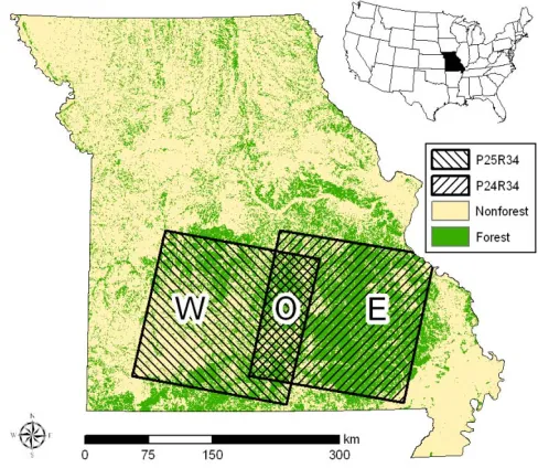
Figure 1: Study areas: Southern Missouri, USA. Data sources: f/nf – USDA Forest Service; base maps – ESRI Data & Maps.

leading to the major rivers. The Springfield plateau is mainly smooth, elevated plains with some dissection due to watercourses (Batek et al., 1999, Foti & Bukenhofer, 1999).

2.2 FIA Data FIA defines forest land as lands cur-rently or formerly supporting a minimum level of tree stocking (10 percent) and not developed for a non-forest use such as agriculture, residential, or industrial use. Forest land includes commercial timberland, some pastured land with trees, forest plantations, unproduc-tive forested land, and reserved, noncommercial forested land. FIA’s definition of forest land also requires a min-imum area of 0.405 ha and minmin-imum continuous canopy width of 36.58 m (U.S. Department of Agriculture Forest Service, 2003). FIA sample plots follow a nationally con-sistent configuration comprised of a cluster of four fixed-radius circular subplots, selected from a nationally con-sistent hexagonal sampling frame with at least one plot selected for each 2400-ha hexagon (Bechtold & Scott, 2005, Reams et al., 2005). On each FIA plot, land use (e.g., proportion forest cover), tree (e.g., species, height, and diameter at breast height: DBH, 1.37 m) and other site variables are collected.

The FIA database was queried to obtain inventory field plot data collected between 1999 and 2007 within all Missouri counties intersecting P25R34 and P24R34. Ge-ographic information system (GIS) data layers of

inven-tory plot center locations were created based on global positioning system (GPS) coordinates obtained during field data collection. GPS coordinates were collected and maintained in North American Datum of 1983. The FIA plots were further constrained to retain only those plots located within the geographic extent of P25R34 or P24R34. FIA plots measured during Missouri cycle 5 (1999-2003) were used for analyses across space (n = 2320), with 751 plots within W, 1278 plots within E and 291 plots within O (Fig. 1). P25R34 plots measured during cycle 5 and remeasured during cycle 6 (2004-2007) were used for analyses across time (n=735). FIA plots from cycle 6 were not used for modeling within P24R34. For each plot, estimates were produced for 1) proportion forest land; and 2) total aboveground gross biomass oven dry weight per hectare on forest land, based on trees 2.54 cm diameter or larger, including all tops and limbs, but excluding foliage (DRYBIOT in FIA database, hereafter: ‘biomass’). Biomass is calculated as per Heath et al. (2008). The mean, range, and standard deviation of per-plot estimates of biomass (Mg/ha) on forest land for each study area were W - 11.65, 33.44, and 6.70; O - 12.19, 32.21, and 6.30; and E - 13.41, 39.15, and 6.45; respectively.

2.3 Satellite Imagery WRS-2 Landsat image

frames overlap across both “paths,” which reflect the roughly north-south track of the satellites, and “rows”, which are segments of paths approximately 185-km in length. Cross-path comparisons were selected because substantial overlap only exists for adjacent paths (Guindonet al., 2004).

For comparisons across space, a Landsat 5 Thematic Mapper (TM) image was obtained for P25R34, dated 29 August 2000; and a Landsat 7 ETM+ image was ob-tained for P24R34, dated 30 August 2000 (Fig. 2). Com-parisons across time were conducted within P25R34, us-ing the 29 August 2000 TM image and a TM image from 2 September 2007. Resulting images had 28.5-m x 28.5-m spatial resolution and Universal Transverse Mer-cator (UTM) projection, with North American Datum of 1983. Clouds and cloud shadows, which covered a mini-mal fraction of the study area, were manually delimited and these areas were excluded from further analyses.

Figure 2: Landsat images of P25R34 (left) and P24R34 (right), late August 2000, southern Missouri, USA.

surface reflectance comparable to the standard MODIS reflectance product (the greater of 0.5 percent absolute reflectance or 5 percent of the recorded reflectance value; Masek, et al., 2006). This pre-processing has been a standard component of the NAFD project (Goward et al., 2008). No further empirical or theoretical normal-ization was performed.

In addition to Landsat surface reflectance data, two topographic layers were also used for prediction and mapping. The first was eleva-tion from the 1 Arc Second National Elevation Dataset, assembled by the U.S. Geological Survey (http://seamless.usgs.gov/products/1arc.php). The second was direct, clear-sky shortwave radiation, which was based on the above elevation dataset and a routine described by Kumar et al. (1997), incorporating a solar date within the range of Landsat acquisitions.

3

Methods

We created models using NAFD image data and as-sessed their performance using validation input from: 1) the same image as the original model; 2) an adjacent, overlapping Path/Row image from the same year, e.g., performance across space; and 3) the same Path/Row, but from a different year, having a similar anniversary date, e.g., performance across time. Descriptions of the RF modeling process used, as well as the specific tests, are below.

3.1 Random Forests RF uses a collection of tree-structured classifiers{h(x,Θk), k = 1,. . . ,}where x is an input pattern and{Θk} are independent identically distributed random vectors. A split for each node is de-termined by training each tree in RF on a bootstrapped sample of the original training data, across a randomly selected subset of the input variables. For classification,

each tree in the RF casts a unit vote. The most popular class at input x determines the classification (Breiman, 2001).

RF combines bagging (bootstrap aggregating) with random feature selection for decision trees (Breiman, 2001). Bagging involves the generation of different train-ing sets drawn randomly from the original data set, with replacement, and combining the resulting classifier deci-sions using a majority vote with equal weight (Breiman, 1996a). Within RF the original sample is partitioned into subsamples, forming node splits until end nodes re-sult, each of which represents a particular class (Watts et al., 2009). Splitting results in a ‘forest’ of classifica-tion trees, each of which can differ greatly from the next. Final classification is determined by an ‘among-tree plu-rality decision’, based on votes cast by each tree in the forest. Out-of-bag (OOB) accuracy measures are pro-duced by withholding a random subset of the original data from the modeling process, and using that OOB data for estimating model accuracy of the classification trees (Lawrence et al., 2006).

Applications of RF for estimation are similar to those described above for classification, but for regression ap-plications, the final prediction is derived from the av-erage of the suite of individual tree outputs (Breiman, 2001).

3.2 Per-pixel predictionsNAFD protocols include methods for making spatially explicit (map-based) esti-mates of changes in aboveground forest biomass (Healey et al., 2007, Powell et al., 2010). Per-pixel predictions of biomass and forest probability were produced using RF models. The work reported here was done with R statistical software (R Development Core Team, 2008) using an implementation of RF developed by Liaw and Wiener (2002) and adapted by Freeman and Frescino (2008). This adaptation applies RF models to pixels in a raster image (ERDAS Imagine format) that corre-sponds to the input satellite imagery. For this approach, 2000 trees were created, with each tree using a different random subset of the data. The number of predictors tried at each node was optimized using the “tuneRF()” function (Freeman and Frescino, 2008). These trees were assembled into a ‘forest’ and each tree provided a ‘vote’ on the final, composite tree. Pixels with predictions of forest probability of 0.5 or greater were labelled forest class; all other pixels were labelled non-forest.

larger. Sixty percent of the FIA plots within W and E and 40 percent of the FIA plots within O were selected at random as training data for P25R34 models. The re-maining 40 percent of plots within W and E (n=300 and 511, respectively) and 60 percent of plots within O (n = 175) were retained for validation analyses. A model for P25R34 was applied to: 1) spectral data from WO (i.e., image pixels from the same image for which the model was developed); and 2) spectral data from EO (i.e., image pixels from the adjacent image - P24R34). The same set of FIA validation plots from O was used to assess both applications of the model.

The procedure was duplicated exactly with data from scene E to create predicted maps of biomass and for-est proportion in area O using imagery from both W and E, thus allowing for comparison of predictions over the same area made with two different imagery sources. Within O, the same model and validation plots were used for both P25R34 and P24R34 models and valida-tion tests.

3.2.2 Predictions Across Time For the year 2000 model, 60 percent of the FIA plots from Missouri cycle 5 (1999-2003) were selected at random for model develop-ment and the remaining 40 percent of plots (n 300) were retained for model validation. Similarly, for the year 2007 model, 60 percent of the FIA plots from Missouri cycle 6 (2004-2007) were selected at random for model development and the remaining 40 percent of plots (n 300) were retained for model validation.

A model based on 2000 imagery was applied to: 1) spectral data from 2000 (i.e., image pixels from the same image for which the model was developed); and 2) spec-tral data from 2007. Similarly, a model based on 2007 imagery was applied to: 1) spectral data from 2007 (i.e., image pixels from the same image for which the model was developed); and 2) spectral data from 2000.

3.3 Validation Quantitative assessment of product accuracies is a prerequisite to acceptance and applica-tion of image-based classificaapplica-tion and estimaapplica-tion prod-ucts (Congalton, 2004). Areas of overlap between adja-cent path/row pairs of satellite images provide not only for “chain classification” of adjacent images (Knorn et al., 2009), but also for quasi-independent validation of classification or estimation. Classification consistency, determined by comparing overlapping portions of in-dividual path/row scenes, can be used as an indicator of classification quality (Cihlar et al., 2003, Guindon & Edmonds, 2004). Extensive image overlap exists for most land resources satellites (e.g., Landsat). In addi-tion to assessing classificaaddi-tion consistency, image overlap regions have been used to characterize the accuracy of landscape metrics (Brown et al., 2000) and systematic

surface reflectance and leaf area index (Butson & Fer-nandes, 2004).

We compared model-based site-specific (per-pixel) classifications of f/nf classification and predictions of biomass with independent ground reference data. When comparing models across space and across time, a nam-ing convention is employed whereby the first term refers to the image source for model development, and the sec-ond term refers to the imagery for which models are im-plemented. Across-space comparisons are termed W-E or E-W, and across-time comparisons are termed 2000-2007, or 2007-2000. Model validation is termed W-W, E-E, 2000-2000, or 2007-2007 when using the same im-age source for model development and testing.

Site-specific validation tests of f/nf classification were conducted to assess overall classification accuracy and Cohen’s kappa coefficient, both of which are based on a confusion matrix of observed and predicted values (Cohen, 1960). Model predictions were compared to FIA validation plot observations. Kappa analysis pro-vides two statistical tests of significance. The first tests whether a classification (e.g., satellite image-based f/nf classification) is significantly better than a classification generated by randomly assigning class labels to image pixels. In the second Kappa test, confusion matrices from two classification maps can be compared to deter-mine whether they are statistically significantly differ-ent from one another (Bishop et al., 1975). Although remotely sensed data are discrete, Cohen’s kappa coeffi-cient is asymptotically normally distributed (Congalton & Green, 2008).

The following test statistics were obtained for the f/nf classification: 1) overall accuracy, 2) maximum likeli-hood estimate of Kappa, 3) approximate large sample variance of Kappa, 4) significance test of a single confu-sion matrix, and 5) a test statistic for testing whether two independent confusion matrices are significantly dif-ferent (Congalton & Green, 2008, Hudson & Ramm, 1987). As for predictions of f/nf class, predictions of biomass were compared to FIA validation plot observa-tions, resulting in estimates of coefficient of determina-tion (R2) and RMSE,

RMSE =

1

n

n

i=1

(ˆy_i−y_i)2 ₍₁₎

4

Results

4.1 Across Space Comparing image surface re-flectance values collected one day apart, but from dif-ferent satellite sensors, (Landsat 5 TM vs. Landsat 7 ETM+), we noted the following correlation coefficients for TM/ETM+ bands 1-5 and 7, respectively, for a sam-ple of pixels that contained FIA plot locations: 0.95, 0.96, 0.97, 0.94, 0.97, and 0.97. The three visible bands – 2, 3, and 1, respectively and in order, appeared most important for classifying f/nf, as determined by both mean square error (MSE) and node purity (gini coeffi-cient) (Breiman et al., 1984). For biomass estimation, at least two of the near/mid-infrared bands (4, 5, and 7) appeared among the three most important attributes, both for MSE and for node purity. For both f/nf classi-fication and biomass estimation, the ancillary attributes of elevation and radiation appeared to be the least im-portant attributes, for both MSE and node purity.

Models of f/nf classification for O - the overlapping portion of P24R34 and P25R34 - resulted in area esti-mates ranging from 44.1 to 50.8 percent for non-forest class and 49.2 to 55.9 percent of forest class (Table 1). Overall accuracy of the f/nf models ranged from 92 to 94 percent, and estimates of Cohen’s kappa coefficients ranged from 0.84 to 0.88, with variances ranging from 0.00131 to 0.00164 and Z statistics ranging from 24.2 to 20.8, all of which are statistically significant at the α=0.05 level (Z<1.96) (Table 1).

Pairwise comparisons of f/nf classifications resulted in Z statistics ranging from 0.03 to 0.629, all of which represent statistically non-significant differences at the α=0.05 level (Z<1.96).

Biomass models had R2 values of 0.72 to 0.74, and RMSEp values of 0.56 to 0.60. In some cases, applying a model based on imagery from one path/row to im-agery in the adjacent, overlapping path/row resulted in slightly higher accuracies (Fig. 3).

4.2 Across Time Area estimates of non-forest and forest in P25R34 ranged from 60.9 to 61.6 and 38.4 to 39.1 percent of the study area, respectively, for 2000 and 2007 (Table 2). Overall accuracies of f/nf classifications ranged from 88 to 90 percent (Table 2). Cohen’s kappa coefficients, variances, and Z statistics ranged from 0.762 to 0.790, 0.00126 to 0.00140, and 20.4 to 22.3, respec-tively, all of which are statistically significant at the α =0.05 level (Z<1.96) (Table 2).

Z statistics ranged from 0.134 to 0.529 for pairwise comparisons of f/nf classifications for P25R34 during 2000 and 2007, all of which represent statistically non-significant differences at theα=0.05 level (Z<1.96).

Biomass models for P25R34 had R2 values of 0.74 to 0.79, and RMSEp values of 0.64 to 0.72 (Fig. 4).

Differ-0 0.2 0.4 0.6 0.8 1

W-W W-E E-W E-E

T

e

st

st

a

ti

s

ti

c

Model-Test Forest biomass

R²

RMSE (prop. of mean)

Figure 3: Error metrics for predictions of forest biomass, 2000, southern Missouri, USA.

ences between the models built in 2000 and 2007 were negligible relative to 2000 and 2007 test data. In some cases, the ”off year” models were fractionally better than models produced in the same year (Fig. 4).

5

Discussion

In this study, satellite-based models of biomass and f/nf classification were applied both to input images used to develop the models and to other images not used to develop the models. Results for overall accuracy of f/nf classification (92 - 94 percent) were among the larger val-ues reported for f/nf classification studies, e.g., 88 per-cent for a k-Nearest Neighbor classification of f/nf/water in northern Minnesota, USA (Haapanen et al., 2004), and 96 percent for an SVM classification of f/nf in the Carpathian Mountains of central Europe (Knorn et al., 2009). Results for RMSEp (0.56 – 0.60) were similar to, or slightly smaller than reported for other studies, e.g., 0.68 – 0.87 for Arizona, USA and 0.61 – 0.69 for Minnesota, USA study areas (Powellet al., 2010).

state-Table 1: Comparison of f/nf classifications for models developed using imagery and plot data from either path/row and applied to imagery from the same path/row or to imagery in the same row and adjacent path, 2000, southern Missouri, USA.

Model / Application

Non-forest (%)

Forest (%)

Overall Accuracy (%)

Cohen’s Kappa Coefficient

Variance of Kappa

Z Statistic

W-W 44.1 55.9 93.8 0.874 0.00135 23.8

W-E 49.2 50.8 92.1 0.842 0.00164 20.8

E-W 49.7 50.3 93.8 0.876 0.00131 24.2

E-E 50.8 49.2 92.7 0.853 0.00152 21.9

Table 2: Comparison across time of f/nf classifications, Path 25 / Row 34, for models developed using imagery and plot data from either 2000 or 2007 and applied to imagery from the same year and to imagery from the alternate year, southern Missouri, USA.

Model / Application

Non-forest (%)

Forest (%)

Overall Accuracy (%)

Cohen’s Kappa Coefficient

Variance of Kappa

Z Statistic

2000-2000 61.3 38.7 89.2 0.783 0.00129 21.8

2000-2007 61.6 38.4 88.9 0.776 0.00133 21.3

2007-2000 60.9 39.1 89.6 0.790 0.00126 22.3

2007-2007 61.6 38.4 88.2 0.762 0.00140 20.4

of-the-art radiometric correction was applied to all im-agery. While these conditions undoubtedly contributed to successful transfer of models across image acquisi-tions, we are encouraged that such measures already are becoming standard procedure in major mapping efforts, e.g., NAFD.

Consistency of these results implies a consistency of both Landsat satellite imagery and FIA data across space and time, even when imagery from two different Landsat sensors was utilized. Results of this study sug-gest that RF can be used with FIA plot data and Land-sat images for modeling f/nf classifications and biomass across time, even for years of imagery when no inventory plot data are available. Furthermore, f/nf classification and biomass prediction appear to be consistent across overlapping image paths, and between Landsat TM and ETM+ images, allowing for flexibility in image selection and compositing over large geographic extents.

The implication of this work is that, at least for for-est types similar to those studied here, different image acquisitions may be combined within the same forest modeling framework with little loss of accuracy. Cross-acquisition model stability leads to several operational mapping advantages. Spectral relationships were not tested here across major ecological or edaphic bound-aries, but results suggested that at least within ecosys-tems, scene-by-scene models of forest structure and pres-ence need not be created. Combination of the spectral and field data from adjacent scenes will usually mean

that forest models can be supported by more observa-tions. In many cases, increased training data might be expected to lead to more precise or more robust models. Additionally, for geographic extents containing multiple, semi-overlapping images (e.g., Landsat), precedence can be given to those images with the most desirable char-acteristics, e.g., least cloud cover or having acquisition date closest to a prescribed anniversary date.

Equally important, results suggested that an assess-ment of model accuracy using imagery and field data from one time period roughly corresponds to the accu-racy of maps created when that same model is applied to properly calibrated imagery from other time periods. This is important because although relatively consistent Landsat imagery is available for many locations since ap-proximately 1985, consistently collected, geo-referenced validation data is rarely available for early dates. In addition to supporting development of maps showing historic forest conditions, application of models to time series of imagery may also enhance forest change detec-tion.

0 0.2 0.4 0.6 0.8 1

2000-2000 2000-2007 2007-2000 2007-2007

T

e

st

s

tat

is

ti

c

Model-Test Forest biomass

R²

RMSE (prop. of mean)

Figure 4: Error metrics for predictions of forest biomass, P25R34, southern Missouri, USA.

to forest probability for labelling as forest those pixels having a probability of 0.5 or greater; all others were labelled non-forest. This “hard” boundary was compa-rable to using an RF categorical model for classification. In applications outside of the context of the current com-parison, however, modeling forest as a continuous prob-ability allows flexible threshold determination in light of classification accuracy based on the kappa statistic, the area under the receiver operating characteristic curve, or a number of other measures.

This study focused on a relatively small geographic extent within central USA. Caution should be exercised when extrapolating these conclusions to other areas. We recommend replication of this study in other geographic regions to test model consistency across space and time.

6

Conclusions

This work confirms that careful image selection and radiometric correction can enable the historical archive of Landsat satellite imagery to be treated interchange-ably for the modeling and mapping of forest character-istics. This finding is useful both in the training and validation stages of model- and map-making. If the in-clusion of adjacent images in the same modeling frame allows the inclusion of more ground data in the train-ing process, resulttrain-ing model predictions will presumably tend to be more robust and possibly more precise. There may also be time savings if forest composition and struc-ture do not need to be modeled separately for each in-dividual scene.

The validation advantages of the image inter-changeability suggested by this work are particularly acute when models are applied over time. Although comprehensive historical ground data are unavailable in many areas, this work suggests that if images are care-fully chosen and calibrated, error rates found in the model-building phase are good indicators of the accu-racy of maps that may be created when those models are applied to historic imagery.

Acknowledgements

References

Baccini, A., Friedl, M. A., Woodcock, C. E. & Warbing-ton, R. (2004) Forest biomass estimation over regional scales using multisource data. Geophysical research letters,31,L10501, doi:10510.11029/12004GL019782.

Baccini, A., Laporte, N., Goetz, S. J., Sun, M. & Dong, H. (2008) A first map of tropical Africa’s above-ground biomass derived from satellite imagery. Envi-ronmental Research Letters,4,9.

Batek, M. J., Rebertus, A. J., Schroeder, W. A., Haith-coat, T. L., Compas, E. & Guyette, R. P. (1999) Re-construction of early nineteenth century vegetation and fire regimes in the Missouri Ozarks. Journal of Biogeography,26,397-412.

Bechtold, W. A. & Scott, C. T. (2005) The forest in-ventory and analysis plot design, In: Bechtold, W. A. & Patterson, P. L. (eds.) The enhanced forest in-ventory and analysis program - national sampling de-sign and estimation procedures. U.S. Department of Agriculture Forest Service, Asheville, NC. pp. 27-42. Available at: http://www.treesearch.fs.fed.us/pubs/ 20378

Behrens, T., Schmidt, K., Zhu, A. X. & Scholten, T. (2009) The conmap approach for terrain-based digital soil mapping.European Journal of Soil Science,9999.

Bishop, Y. M., Fienberg, S. E. & Holland, P. W. (1975) Discrete multivariate analysis - theory and practice. MIT Press, Cambridge, MA, pp.

Breiman, L. (1996a) Bagging predictors.Machine Learn-ing,24,123-140.

Breiman, L. (1996b) Stacked regressions. Machine Learning,24,49-64.

Breiman, L. (2001) Random Forests.Machine Learning, 45,5-32.

Breiman, L., Friedman, J. H., Olshen, R. A. & Stone, C. J. (1984)Classification and regression trees. Wadsworth International Group, Belmont, California, 358pp.

Brown, D. G., Duh, J.-D. & Drzyzga, S. A. (2000) Es-timating error in an analysis of forest fragmentation change using north american landscape characteriza-tion (nalc) data.Remote Sensing of Environment,71, 106-117.

Butson, C. R. & Fernandes, R. A. (2004) A consistency analysis of surface reflectance and leaf area index re-trieval from overlapping clear-sky Landsat ETM+ im-agery.Remote Sensing of Environment,89,369-380.

Chan, J. C.-W. & Paelinckx, D. (2008) Evaluation of random forest and adaboost tree-based ensemble clas-sification and spectral band selection for ecotope map-ping using airborne hyperspectral imagery. Remote Sensing of Environment,112,2999-3011.

Cihlar, J., Latifovic, R., Beaubien, J., Trishchenko, A., Chen, J. & Fedosejevs, G. (2003) National scale forest information extraction from coarse resolution satellite data, part 1, In: Wulder, M. A. & Franklin, S. E. (eds.) Remote sensing of forest environments: Con-cepts and case studies. Kluwer Academic Publishers, Boston. pp. 337-357.

Cleland, D. T., Freeouf, J. A., Keys, J., James E., Nowacki, G. J., Carpenter, C. A. & McNab, W. H. (2007) Ecological subregions: Sections and sub-sections of the conterminous United States [geospa-tial dataset]. Compiled at 1:500,000 to 1:1,000,000 scales in participation with federal and state agen-cies and nongovernmental partners. U.S. Department of Agriculture, Forest Service: Eastern Region, Mil-waukee, WI; Rocky Mountain Region, Lakewood, CO; Washington Office, Washington, DC; Northeastern Area State and Private Forestry, Durham, NH; South-ern Research Station, Ashville, NC. Available online at: http://svinetfc4.fs.fed.us/clearinghouse/other resources/ecosubregions.html, last accessed 23 De-cember 2010.

Cohen, J. (1960) A coefficient of agreement for nominal scales. Educational and Psychological Measurement, 20,37-46.

Cohen, W. B. & Goward, S. N. (2004) Landsat’s role in ecological applications of remote sensing. Bioscience, 54,535-545.

Congalton, R. G. (2004) Putting the map back in map accuracy assessment, In: Lunetta, R. S. & Lyon, J. G. (eds.) Remote sensing and GIS accuracy assessment. Taylor & Francis Books, Inc., Boca Raton, FL. pp. 1-11.

Congalton, R. G. & Green, K. (2008)Assessing the accu-racy of remotely sensed data: Principles and practices. (2nd edn), CRC Press, Boca Raton, 183pp.

Cutler, D. R., Edwards, T. C., Beard, K. H., Cutler, A., Hess, K. T., Gibson, J. & Lawler, J. J. (2007) Random forests for classification in ecology. Ecology, 88,2783-2792.

Evans, J. & Cushman, S. (2009) Gradient modeling of conifer species using random forests. Landscape Ecol-ogy,24,673-683.

Foti, T. L. & Bukenhofer, G. A. (1999) Chapter 1: Ecological units of the highlands.In: Ozark-Ouachita Highlands Assessment: terrestrial vegetation and wildlife.Report 5 of 5, Gen. Tech. Rep. SRS-35. U.S. Department of Agriculture, Forest Service, Southern Research Station, Asheville, NC, 1-6 pp.

Freeman, E. & Frescino, T. A. (2008) Modelmap: Mod-eling and map production using random forest and stochastic gradient boosting. Package for ’r’ statistical software. 1.1 ed. Ogden, Utah, USDA Forest Service, Rocky Mountain Research Station.

Gislason, P. O., Benediktsson, J. A. & Sveinsson, J. R. (2006) Random Forests for land cover classification. Pattern Recognition Letters,27,294-300.

Goward, S. N., Masek, J. G., Cohen, W. B., Moisen, G. G., Collatz, G. J., Healey, S., Houghton, R. A., Huang, C., Kennedy, R., Law, B., Powell, S., Turner, D. & Wulder, M. A. (2008) Forest disturbance and North American carbon flux. Eos, Transactions American Geophysical Union,89,105-116.

Guindon, B. & Edmonds, C. M. (2004) Using classifica-tion consistency in inter-scene overlap areas to model spatial variations in land-cover accuracy over large ge-ographic regions, In: Lunetta, R. S. & Lyon, J. G. (eds.) Remote sensing and GIS accuracy assessment. Taylor & Francis Books, Inc., Boca Raton, FL. pp. 133-144.

Haapanen, R., Ek, A. R., Bauer, M. E. & Finley, A. O. (2004) Delineation of forest/nonforest land use classes using nearest neighbor methods. Remote Sensing of Environment, 89,265-271.

Hme, T., Stenberg, P., Andersson, K., Rauste, Y., Kennedy, P., Folving, S. & Sarkeala, J. (2001) AVHRR-based forest proportion map of the pan-european area. Remote Sensing of Environment, 77, 76-91.

Hansen, M. C., DeFries, R. S., Townshend, J. R. G., Carroll, M., Dimiceli, C. & Sohlberg, R. A. (2003) Global percent tee cover at a spatial resolution of 500 meters: First results of the MODIS vegetation contin-uous fields algorithm.Earth Interactions,7,1-15.

Healey, S. P., Moisen, G., Masek, J., Cohen, W., Goward, S., Powell, S., Nelson, M., Jacobs, D., Lis-ter, A., Kennedy, R. & Shaw, J. (2007) Measurement of forest disturbance and re-growth with Landsat and FIA data: Anticipated benefits from forest inventory and analysis’ collaboration with the national aeronau-tics and space administration and university partners. In: McRoberts, R. E., Reams, G. A., Van Deusen, P. C. & McWilliams, W. H. (eds.)Proceedings of the Sev-enth Annual Forest Inventory and Analysis Sympo-sium, Portland, ME, 3-6 October 2005. Available on-line at: http://www.treesearch.fs.fed.us/pubs/30424

Healey, S. P., Yang, Z., Cohen, W. B. & Pierce, D. J. (2006) Application of two regression-based methods to estimate the effects of partial harvest on forest struc-ture using Landsat data.Remote Sensing of Environ-ment,101,115-126.

Heath, L. S., Hansen, M. H., Smith, J. E., Miles, P. D. & Smith, W. B. (2008) Investigation into calculating tree biomass and carbon in the FIADB using a biomass expansion factor approach. In: McWilliams, W. H., Moisen, G. G. & Czaplewski, R. L. (eds.) 2008 For-est Inventory and Analysis (FIA) Symposium, Park City, UT, 21-23 October 2008. Available online at: http://www.treesearch.fs.fed.us/pubs/33351

Hudak, A. T., Crookston, N. L., Evans, J. S., Hall, D. E. & Falkowski, M. J. (2008) Nearest neighbor impu-tation of species-level, plot-scale forest structure at-tributes from LiDAR data. Remote Sensing of Envi-ronment,112,2232-2245.

Hudson, W. D. & Ramm, C. W. (1987) Correct formula-tion of the kappa coefficient of agreement. Photogram-metric Engineering & Remote Sensing,53,421-422.

Kennedy, P. & Bertolo, F. (2002) Mapping sub-pixel for-est cover in europe using AVHRR data and national

and regional statistics. Canadian Journal of Remote Sensing,28,302-331.

Kirschbaum, A. A. (2008)Mapping mortality following a long-term drought in a pinyon-juniper ecosystem in arizona and new mexico using Landsat data. M.S., Oregon State University.

Knorn, J., Rabe, A., Radeloff, V. C., Kuemmerle, T., Kozak, J. & Hostert, P. (2009) Land cover mapping of large areas using chain classification of neighboring Landsat satellite images.Remote Sensing of Environ-ment,113,957-964.

Kumar, L., Skidmore, A. K. & Knowles, E. (1997) Mod-elling topographic variation in solar radiation in a GIS environment. International Journal for Geographical Information Science,11,475-497.

Larsson, H. (1993) Linear regression for canopy cover estimation in acacia woodlands using LandsatTM, -MSS, and SPOT HRV xs data.International Journal of Remote Sensing,14,2129-2136.

Lawrence, R. L., Wood, S. D. & Sheley, R. L. (2006) Mapping invasive plants using hyperspectral imagery and breiman cutler classifications (randomforest). Re-mote Sensing of Environment,100,356-362.

LeBlanc, M. & Tibshirani, R. (1996) Combining esti-mates in regression and classification.Journal of the American Statistical Association,91,1641-1650.

Liaw, A. & Wiener, M. (2002) Classification and regres-sion by randomforest.R News,2/3,18-22.

Nelson, M. D., Healey, S. P., Moser, W. K. & Hansen, M. H. (2009) Combining satellite imagery with forest inventory data to assess damage severity following a major blowdown event in northern Minnesota, USA. International Journal of Remote Sensing, 30, 5089– 5108.

Ohmann, J. L. & Gregory , M. J. (2002) Predictive map-ping of forest composition and structure with direct gradient analysis and nearest- neighbor imputation in coastal Oregon, U.S.A. Canadian Journal of Forest Research,32,725-741.

Opitz, D. & Maclin, R. (1999) Popular ensemble meth-ods: An empirical study.Journal of Artificial Intelli-gence Research,11,169-198.

inventory for sustainable forest management and bio-diversity monitoring.(vol. 76) Kluwer Academic Pub-lishers, Dordrecht, The Netherlands. pp. 279-294.

Pal, M. (2005) Random forest classifier for remote sens-ing classification. International Journal of Remote Sensing,26,217-222.

Powell, S. L., Cohen, W. B., Healey, S. P., Kennedy, R. E., Moisen, G. G., Pierce, K. B. & Ohmann, J. L. (2010) Quantification of live aboveground forest biomass dynamics with Landsat time-series and field inventory data: A comparison of empirical model-ing approaches.Remote Sensing of Environment,114, 1053-1068.

Prasad, A., Iverson, L. & Liaw, A. (2006) Newer classi-fication and regression tree techniques: Bagging and Random Forests for ecological prediction.Ecosystems, 9,181-199.

R Development Core Team (2008) R: A language and en-vironment for statistical computing. ISBN 3-900051-07-0 ed. Vienna, Austria, R Foundation for Statistical Computing.

Reams, G. A., Smith, W. D., Hansen, M. H., Bech-told, W. A., Roesch, F. A. & Moisen, G. G. (2005) The forest inventory and analysis sampling frame, In: Bechtold, W. A. & Patterson, P. L. (eds.) The enhanced forest inventory and analysis program - national sampling design and estimation proce-dures. U.S. Department of Agriculture Forest Ser-vice, Asheville, NC. pp. 11-26. Available online at: http://www.treesearch.fs.fed.us/pubs/20376

Ruefenacht, B., Finco, M. V., Nelson, M. D., Czaplewski, R. L., Helmer, E. H., Blackard, J. A., Holden, G. R., Lister, A. J., Salajanu, D., Weyer-mann, D. & Winterberger, K. (2008) Conterminous U.S. and Alaska forest type mapping using forest inventory and analysis data. Photogrammetric Engi-neering & Remote Sensing, 74,1379-1388.

Steele, B. M. (2000) Combining multiple classifiers: An application using spatial and remotely sensed

infor-mation for land cover type mapping.Remote Sensing of Environment,74,545-556.

Stone, M. (1974) Cross-validatory choice and assessment of statistical prediction.Journal of the Royal Statisti-cal Society. Series B (MethodologiStatisti-cal),36,111-147.

Strobl, C., Boulesteix, A.-L., Kneib, T., Augustin, T. & Zeileis, A. (2008) Conditional variable importance for random forests.BMC Bioinformatics,9,307.

Strobl, C., Boulesteix, A.-L., Zeileis, A. & Hothorn, T. (2007) Bias in random forest variable importance measures: Illustrations, sources and a solution.BMC Bioinformatics,8,25.

U.S. Department of Agriculture Forest Service (2003) Forest inventory and analysis national core field guide, volume 1: Field data collection procedures for phase 2 plots, version 2.0.In: U.S. Depart-ment of Agriculture, Forest Service, Forest Inven-tory and Analysis, Washington, DC, 281 pp. Available online at: http://www.fia.fs.fed.us/library/database-documentation/

Vapnik, V. N. (2000) The nature of statistical learning theory.(2nd edn), Springer, New York, 314pp.

Watts, J. D., Lawrence, R. L., Miller, P. R. & Mon-tagne, C. (2009) Monitoring of cropland practices for carbon sequestration purposes in north central Mon-tana by Landsat remote sensing. Remote Sensing of Environment,113,1843-1852.

Wolpert, D. (1992) Stacked generalizations.Neural Net-works,5,241-259.

Woodcock, C. E., Macomber, S. A., Pax-Lenny, M. & Cohen, W. B. (2001) Monitoring large areas for forest change using Landsat: Generalization across space, time and Landsat sensors. Remote Sensing of Envi-ronment,78,194-203.