www.theoryofcomputing.org
Time Bounds for Streaming Problems
Raphaël Clifford
∗Markus Jalsenius
†Benjamin Sach
Received March 13, 2017; Revised January 11, 2018; Published September 7, 2019
Abstract: We give tight cell-probe bounds for the time to compute convolution, multipli-cation and Hamming distance in a stream. The cell probe model is a particularly strong computational model and subsumes, for example, the popular word RAM model.
• We first consider online convolution where the task is to compute the inner product between a fixedn-dimensional vector and a vector of thenmost recent values from a stream. One symbol of the stream arrives at a time and then each output symbol must be computed before the next input symbol arrives.
• Next we show bounds for online multiplication of twon-digit numbers where one of the multiplicands is known in advance and the other arrives one digit at a time, starting from the lower-order end. When a digit arrives, the task is to compute a single new digit from the product before the next digit arrives.
• Finally we look at the online Hamming distance problem where the Hamming distance is computed instead of the inner product.
For each of these three problems, we give a lower bound ofΩ((δ/w)logn) time on
average per output symbol, where δ is the number of bits needed to represent an input symbol andwis the cell or word size. We argue that these bounds are in fact tight within the cell probe model.
ACM Classification:F.2.2
AMS Classification:68Q17
Key words and phrases:lower bounds, cell probe, streaming algorithms, online algorithms
Preliminary versions of these results first appeared in the Proceedings of the 38thInternational Colloquium on Automata, Languages and Programming (ICALP), 2011 [7] and the Proceedings of the 24th ACM-SIAM Symposium on Discrete Algorithms (SODA), 2013 [8].
∗Supported by EPSRC Fellowship EP/J019283/1.
1
Introduction
We consider the complexity of three related and fundamental problems: computing the convolution of two vectors, multiplying two integers, and computing the Hamming distance between two strings. We study these problems in an online or streaming context and provide matching upper and lower bounds in the cell-probe model. Time lower bounds in the cell-probe model also hold for the popular word-RAM model in which many of today’s algorithms are given.
The importance of these problems is hard to overstate. The integer multiplication and convolution problems have played a central role in modern algorithm design and theory. The question of how to compute the Hamming distance efficiently has a rich literature, spanning many of the most important fields in computer science. Within the theory community, communication complexity based lower bounds and streaming model upper bounds for the Hamming distance problem have been the subject of particularly intense study [10,35,17,19,4,5]. This previous work has however almost exclusively focused on providing resource bounds either in terms of space or bits of communication rather than time complexity.
We begin by introducing the problems and stating our results. In the following problem definitions and throughout, we write[q]to denote the set{0, . . . ,q−1}, whereqis a positive integer and a parameter of the problem.
Problem 1.1(Online convolution). For a fixed vectorF∈[q]n of lengthn, we consider a stream in
which numbers from[q]arrive one at a time. For each arriving number, before the next number arrives, we compute the inner product (moduloq) ofFand the vector that consists of the most recentnnumbers of the stream.
Theorem 1.2. In the cell-probe model with w bits per cell, for any positive integers q and n, and any randomised algorithm solving the online convolution problem, there exist instances such that the expected amortised time isΩ((δ/w)logn)per arriving value, whereδ =dlog2qe.
Problem 1.3(Online multiplication). Given two numbersF,X∈[qn], whereqis the base andnis the number of digits per number, we want to compute thenleast significant digits of the product ofF andX, in baseq. We must do this under the constraint that onlyFis known in advance and the digits ofX arrive one at a time, starting from the lower-order end. When thei-th digit ofXarrives, before the(i+1)-th digit arrives, we compute thei-th digit of the product.
Theorem 1.4. In the cell-probe model with w bits per cell, for any positive integers q and n, and any randomised algorithm solving the online multiplication problem in base q, there exist instances such that computing the n least significant digits of the product takesΩ((δ/w)nlogn)expected time, where δ=dlog2qe.
Problem 1.5(Online Hamming distance). For a fixed stringF of lengthn, we consider a stream in which symbols from the alphabet[q]arrive one at a time. For each arriving symbol, before the next symbol arrives, we compute the Hamming distance betweenF and the lastnsymbols of the stream.
Our Hamming distance lower bound also implies a matching lower bound for any problem to which Hamming distance can be reduced. The most straightforward of these is onlineL1distance computation, where the task is to compute theL1distance between a fixed vector of integers and the lastnnumbers in the stream. A suitable reduction was shown in [26]. The expected amortised cell probe complexity for the onlineL1distance problem is therefore alsoΩ((δ/w)logn)per output symbol.
One of our main technical contributions is to extend methods designed to give lower bounds on dynamic data structures to the seemingly distinct field of online algorithms. Whereδ=w, for example, we
haveΩ(logn)lower bounds for all three problems. In particular for online multiplication and convolution,
these lower bounds match the best currently known offline upper bounds in the RAM model. As we discuss inSection 1.1, this may be the highest lower bound that can be proved for all the problems we consider without a further breakthrough.
In order to prove our lower bounds we show the existence of probability distributions on the inputs for which we can prove lower bounds on the expected running time of any deterministic algorithm. By Yao’s minimax principle [36] this immediately implies that for every (randomised) algorithm there is a worst-case input such that the (expected) running time is equally high. Therefore our lower bounds hold equally for randomised algorithms as for deterministic ones.
The lower bounds we give are also tight within the cell-probe model. This can be seen by application of reductions described in [12,6]. It was shown there that any offline algorithm for convolution [6] or multiplication [12] can be converted to an online one with at most anO(logn) factor overhead. For details of these reductions we refer the reader to the original papers. In our case, the same approach also allows us to directly convert any cell-probe algorithm from an offline to online setting. An offline cell-probe algorithm for convolution, multiplication or Hamming distance could first read the whole input, then compute the answer. This takesO((δ/w)n)cell probes. We can therefore derive online
cell-probe algorithms which take onlyO((δ/w)nlogn)probes overninput symbols, henceO((δ/w)logn) (amortised) probes per output. This upper bound matches the new lower bounds we give. We summarise this in the following corollary.
Corollary 1.7. The expected amortised cell-probe complexity of the online convolution, multiplication, Hamming distance and L1-distance problems isΘ((δ/w)logn)per arriving value.
One consequence of our results is the first strict separation between the complexity of exact and approximate pattern matching. Online exact matching can be solved in constant time [15] per new input symbol and our new lower bound proves for the first time that this is not possible for Hamming distance.
Another consequence of our results is a new separation between the time complexity of online exact matching and any convolution-based online pattern matching algorithm. Convolution has played a particularly important role in the field of combinatorial pattern matching where many of the fastest algorithms rely crucially for their speed on the use of fast Fourier transforms (FFTs) to perform repeated convolutions. These methods have also been extended to allow searching for patterns in rapidly processed data streams [6,9].
1.1 Previous results and upper bounds in the RAM model
best current deterministic upper bound for offline Hamming distance computation is anO(n√mlogm) time algorithm based on convolutions [2, 22]. In [21] a randomised algorithm was given that takes O((n/ε2)log2n)time which was subsequently modified in [18] toO((n/ε3)logn). Particular interest
has also been paid to a bounded version of this problem called thek-mismatch problem. Here a boundk is given and we need only report the Hamming distance if it is less than or equal tok. In [23], anO(nk) algorithm was given that is not convolution based and usesO(1)-time lowest common ancestor (LCA) operations on the suffix tree ofPandT. This was then improved toO(n√klogk)time by a method that combines LCA queries, filtering and convolutions [3].
The best time complexity lower bounds for online multiplication of twon-bit numbers were given in the 1974 by Paterson, Fischer and Meyer. They presented anΩ(logn)lower bound for multitape Turing
machines [31] and also gave anΩ(logn/log logn)lower bound for thebounded activity machine(BAM).
The BAM, which is a strict generalisation of the Turing machine model but which has nonetheless largely fallen out of favour, attempts to capture the idea that future states can only depend on a limited part of the current configuration. To the authors’ knowledge, there has been no progress on cell-probe lower bounds for online multiplication, convolution or Hamming distance previous to the work we present here.
There have however been attempts to provide offline lower bounds for the related problem of computing the FFT. In [28] Morgenstern gave anΩ(nlogn)lower bound conditional on the assumption
that the underlying field of the transform is the complex numbers and that the modulus of any complex numbers involved in the computation is at most one. Papadimitriou gave the sameΩ(nlogn)lower bound
for FFTs of length a power of two, this time excluding certain classes of algorithms including those that rely on linear mathematical relations among the roots of unity [30]. This work had the advantage of giving a conditional lower bound for FFTs over more general algebras than was previously possible, including for example finite fields. In 1986, Pan [29] showed that another class of algorithms having a so-called synchronous structure must requireΩ(nlogn)time for the computation of both the FFT and convolution.
The fastest known algorithms for both offline integer multiplication and convolution in the word-RAM model requireO(nlogn)time by a well known application of a constant number of FFTs. As a consequence our online lower bounds for these two problems match the best known time upper bounds for the offline problem. As we discussed above, our lower bounds for all three problems are also tight within the cell-probe model for the online problems.
The question now naturally arises as to whether one can find higher lower bounds in the RAM model. This appears as an interesting question as there remains a gap between the best known time upper bounds provided by existing algorithms and the lower bounds that we give within the cell-probe model. However, as we mention above, any offline algorithm for convolution, Hamming distance or multiplication can be converted to an online one with at most anO(logn)factor overhead [12,6]. As a consequence, a higher lower bound thanΩ(logn)for any of these problems would immediately imply a superlinear lower bound
for the offline version of the corresponding problem. This would be a truly remarkable breakthrough in the field of computational complexity as no such offline lower bound is known even for the canonical NP-complete problem SAT.
so far resisted our best attempts. On the other hand, for online Hamming distance, while our lower bound is tight within the model, it is still distant from the time complexity of the fastest known RAM algorithms. The best known online complexity isO(√nlogn)time per arriving symbol [6]. An improvement of the upper bound for Hamming distance computation to meet our new lower bound would also have significant implications. A reduction that is now regarded as folklore tells us that anyO(f(n))time algorithm for computing the Hamming distance between a pattern and all substrings of a text, assuming a pattern of lengthnand a text of length 2n, implies anO(f(n2))time algorithm for multiplying binary (n×n)-matrices over the integers. Therefore anO(logn)-time online Hamming distance algorithm would imply anO(nlogn)offline Hamming distance algorithm, which would in turn imply anO(n2logn)-time algorithm for binary matrix multiplication. Although such a result would arguably be less shocking than a proof of a superlinear offline lower bound for Hamming distance computation, it would nonetheless be a significant breakthrough in the complexity of a classic and much studied problem.
1.2 The cell-probe model
Our bounds hold in the cell-probe model which is a particularly strong computational model that was introduced originally by Minsky and Papert [27] in a different context and then subsequently by Fredman [13] and Yao [37]. A data structure in the cell-probe model consists of a set of memory cells, each storingwbits. When presented with an update, the data structure reads and updates a number of these cells. Similarly, when presented with a query, the data structure reads cells and from their contents, returns the desired answer. These reads and updates are referred to as cell probes and the cost of an update or query operation is simply the number of cells that are probed. As is typical, we will require that the cell sizewis at least of order lognbits. This allows each cell, or a constant number of cells, to hold the address of any location in memory.
This abstraction makes the model very strong, subsuming for instance the popular word-RAM model. In the word-RAM model certain operations on words, such as addition, subtraction and possibly multipli-cation take constant time (see for example [16] for a detailed introduction). Here a word corresponds to a cell. Any time lower bound in the cell-probe model withw-bit cells gives an asymptotically equal time lower bound in the word-RAM model withw-bit words. This is because each constant-time operation in the word-RAM model only probes a constant number of cells.
The generality of the cell-probe model makes it particularly attractive for establishing lower bounds for dynamic data structure problems and many such results have been given in the past couple of decades. The approaches taken had historically been based only on communication complexity arguments and the chronogram technique of Fredman and Saks [14]. However in 2004, a breakthrough lead by Pˇatra¸scu and Demaine gave us the tools to seal the gaps for several data structure problems [34] as well as giving the firstΩ(logn)lower bounds. The new technique is based on information-theoretic arguments
that we also deploy here. Pˇatra¸scu and Demaine also presented ideas which allowed them to express more refined lower bounds such as trade-offs between updates and queries of dynamic data structures. For a list of data structure problems and their lower bounds using these and related techniques, see for example [32]. A new lower bound of Ω (logn/log logn)2 was given by Larsen in 2012 for the
cell-probe complexity of performing queries in the dynamic range counting problem [24]. This result holds under the natural assumptions ofΘ(logn)-size words and polylogarithmic time updates and is
the field, anΩ((log1/2n/log logn)3) time lower bound for the unweighted version of dynamic range
counting was given which holds even overF2[25].
1.3 Technical contributions
We use one of the most important techniques for proving data structure lower bounds called theinformation transfer methodof Pˇatra¸scu and Demaine [33,34]. For a pair of adjacent intervals of arriving values in the stream, the information transfer is the set of memory cells that are written during the first interval and read in the next interval. These cells must containallthe information from the updates during the first interval that the algorithm needs in order to produce correct output in the next interval. If one can prove that this quantity is large for many pairs of intervals then the desired lower bound follows. To do this we relate the size of the information transfer to the conditional entropy of the output in the relevant interval. The main task of proving lower bounds reduces to that of devising a hard input distribution for which output symbols have high entropy conditioned on selected previous values of the input.
Although the use of information transfer to provide time lower bounds for data structure problems is not new, applying the method to our new online setting has required a number of new insights. At the simplest level, where a standard data structure problem has a number of different possible queries, in our setting there is only one query which is to return the latest result as soon as a new symbol arrives. As a result we provide a complete description of the information transfer method in a form which is relevant to this different setting. At a more detailed mathematical level, perhaps the most surprising innovation we present is a new relationship between the Hamming distance, vector sums and constant-weight binary cyclic codes.
For the three problems we consider, our key contribution is the design of a fixed vector or stringF which together with some random distribution over possible input streams provide a lower bound for the information transfer between successive intervals. For the convolution and multiplication problems we show that a randomly pickedFhas a good chance of being suitable for proving the lower bounds. We also give an explicit description of a particularFfor which the lower bounds are obtained when the values of the input stream are drawn independently and uniformly at random. The vectorF is easy to describe and naturally yields large conditional entropy of the output symbols for intervals of power-of-two lengths.
The results of the convolution and multiplication problems can be seen as a first step towards the lower bound for the Hamming distance problem. Here the stringF is derived by a sequence of transformations. These start with binary cyclic codes and go via binary vectors with many distinct sums and an intermediate string to finally arrive atF itself. The use of such a purposefully designed input departs from the closely related work of the convolution and multiplication lower bounds and also from much of the lower bound literature where simple uniform distributions over the whole input space often suffice.
a hard instance is non-constructive and involves a number of new insights, combining ideas from coding theory and additive combinatorics.
When computing the Hamming distance there is a balance between the number of symbols being used and the length of the strings. For large alphabets and short strings, one would expect a typical Hamming distance to be close to the length of the string on random input symbols and therefore to provide very little information about the random string itself. This suggests that the length of the strings must be sufficiently long in relation to the alphabet size to ensure that the entropy of the output symbols is large, as required by the information transfer method. At first glance, it is not immediately obvious that large entropy can be obtained unless the fixed stringFisexponentiallylarger than the alphabet size. This potentially poses another problem for the information transfer method, namely that a word sizewof order lognwould be much larger thanδ (the number of bits needed to represent a symbol), making a lognlower bound
impossible to achieve.
Our main technical contribution is to show that fixed strings of length only polynomial in the size of the alphabet exist which provide output symbols of sufficiently high entropy. Such strings, when combined with a suitable input distribution maximising the number of distinct Hamming distance output sequences, give us the overall lower bound. We design a fixed stringF with this desirable property in such a way that there is a one-to-one mapping between many of the different possible input streams and the computed Hamming distances. This in turn implies large entropy. The construction ofFis non-trivial and we break it into smaller building blocks, reducing our problem to a purely combinatorial question relating to vectors sums. That is, given a relatively small setV of vectors of lengthm, how many distinct vector sums can be obtained by choosingmvectors fromV and adding them. We show that even if we are restricted to picking vectors only from subsets ofV, there exists aV such that the number of distinct vector sums ismΩ(m). We believe this result is interesting in its own right. Our proof for the combinatorial
problem is non-constructive and probabilistic, using constant-weight cyclic binary codes to prove that there is a positive probability of the existence of a setV with the desired property.
1.4 Organisation
InSection 2we introduce notation and describe the setup for proving the lower bounds. InSection 3we prove the lower bounds for all three problems that we consider. The proofs hinge on a set of lemmas which give lower bounds related to the entropy of the outputs of the problems considered. These lemmas are proven separately in subsequent sections. InSection 4we deal with the lemmas related to the convolution problem, and inSection 5we deal with the lemmas related to the multiplication problem. Finally, in Sections6,7and8we prove the lemma related to the Hamming distance problem.
2
Basic setup for the lower bounds
2.1 The framework
There is afixed array F and an arraySwhich is referred to as thestream. BothF andSare of lengthn and over the set[q]of integers, and we letδ =dlogqedenote the number of bits required to encode a
value from[q]. The valueq, or alternativelyδ, is a parameter of the problem. The problem is to maintain
Ssubject to an update operationUPDATE(x)which takes a symbolx∈[q], modifiesSby appendingxto the right of the rightmost symbolS[n−1]and removing the leftmost symbolS[0], and then outputs the value of a function ofFand the updatedS. In theconvolutionproblem the output is the inner product ofFandS, that is∑i∈[n](F[i]·S[i]), and in theHamming distanceproblem the output is the number of
positionsi∈[n]such thatF[i]6=S[i].
We letU∈[q]ndenote theupdate arraywhich describes a sequence ofn
UPDATEoperations. That is, for eacht∈[n], the operationUPDATE(U[t])is performed. We will usually refer totas thearrivalof
the valueU[t]. Observe that just after the arrivalt, the valuesU[t+1,n−1]are still not known to the algorithm. Finally, we let the length-narrayAdenote the outputs such that fort∈[n],A[t]is the output of
UPDATE(U[t]).
In themultiplicationproblem we letFdenote one of the two operands to be multiplied, henceFis fixed and known in advance by the algorithm. Specifically we letF[i]denote thei-th least significant digit. We letUbe the unknown operand so thatU[t]is itst-th least significant digit. Prior to the arrival of the first digitU[0], the streamScontains only zeros. The outputA[t]is thet-th digit in the product ofF andS, which is a function ofFandU[0,t]as required.
2.2 Hard distributions
Our lower bounds hold for any randomised algorithm on its worst case input. This will be achieved by applyingYao’s minimax principle[36]. That is, we develop lower bounds that hold for any determinis-tic algorithm on some random input. The basic approach is as follows: we devise a fixed arrayFand describe a probability distribution fornnew values arriving in the streamS. We then obtain a lower bound on the expected running time for any deterministic algorithm over these arrivals. Due to the minimax principle, the same lower bound must then hold for any randomised algorithm on its own worst case input. The amortised bound is obtained by dividing byn.
From this point onwards we consider an arbitrary deterministic algorithm running with some fixed arrayFon a random input ofnvalues. The algorithm may depend onF. We refer to the choice ofFand distribution onU as ahard distributionsince it is used to show a lower bound.
2.3 Information transfer
0 1 2 3 4 5 6 7 8 9 10 11 12 13 14 15
v
16 17 18 19 20 21 22 23 24 25 26 27 28 29 30 31
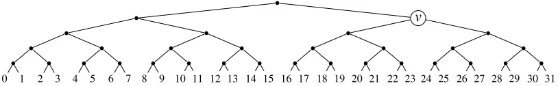
Figure 1: An information transfer treeTwithn=32 leaves. For the node labelledv, the arrival times t0=16,t1=23 andt2=31.
We define the subarrayUv=U[t0,t1]to represent the`v/2 values arriving in the stream during the arrival interval[t0,t1], and we define the subarrayAv=A[t1+1,t2]to represent the`v/2 output symbols produced during the arrival interval[t1+1,t2].
We defineUevto be the concatenation ofU[0,(t0−1)]andU[(t2+1),(n−1)]. That is,Uevcontains all
symbols ofUexcept for those inUv. WhenUevis fixed to some constantuevandUvis random, we write H(Av|Uev=uev)to denote the conditional entropy ofAvunder the fixedUev.
We define theinformation transferof a nodevofT, denotedIv, to be the set of memory cellscsuch
thatcis probed during the interval[t0,t1]and also probed in [t1+1,t2]. The cells in the information transferIvtherefore contains all the information about the values inUvthat the algorithm uses in order to
correctly produce the output symbolsAv.
By adding up the sizes of the information transfersIvover the internal nodesvofTwe get a lower
bound on the number of cell probes, that is a lower bound on the total running time of the algorithm. To see this it is important to make the observation that a particular cell probe is counted for only once. Suppose that the cellc∈Ivfor some nodev. Letpbe the first probe ofcin the arrival interval[t1+1,t2]. By including the cellc∈Ivin the cell probe count we are in fact counting the probep. Now observe that pcannot be counted for in the information transferIv0 of any nodev0wherev0is a proper descendant or
ancestor ofv.
Since the concept of the size of the information transfer is central to the lower bound proofs, we define as a shorthandIv=|Iv|to denote the size of the information transfer.
Definition 2.1(Large expected information transfer). A nodevofThaslarge information transferif
E[Iv] ≥
k·δ·`v
w ,
wherekis a constant that depends on the problem and input distribution.
Our aim is to show that a substantial proportion of the nodes ofThave large information transfer. As we will see inSection 3, this will be achieved by relating the size of the information transfer,Ivto the
entropy of the output symbolsAv.
3
Overall proofs of the lower bounds
onU, conditioned on the fixed value ofUev. This induces a distribution on the output symbolsAv. If
the entropy ofAv is large, conditioned on the fixedUev, then any algorithm must probe many cells in
order to correctly produce the output symbolsAv, as it is only through the information transferIvthat
the algorithm can know anything aboutUv. We will begin inSection 3.1by making this claim precise
by giving a problem independent upper bound onH(Av|Uev=uev)in terms ofIv. We will then give
lower bounds onH(Av|Uev=uev) inSection 3.2 for each problem we consider. The proofs of these
entropy lower bounds form the heart of our contributions and are deferred to Sections4onwards. In
Section 3.3, we combine the upper and lower bounds on the entropy to show that many nodes ofThave large information transfer. Finally, we calculate our final lower bounds inSection 3.4by summing over all large information transfer nodes as discussed inSection 2.3above.
3.1 An upper bound on the entropy
Towards showing that high conditional entropyH(Av|Uev=uev)implies large information transfer we
use the information transferIvto describe an encoding of the output symbolsAv. The following lemma
gives a direct relationship between the size of the information transferIvand the entropy. The lemma was
originally stated in [34] but for completeness we restate it here in our notation and provide a full proof.
Lemma 3.1(Pˇatra¸scu and Demaine [34]). Under the assumption that the address of any cell can be specified in w bits, for any node v of the information transfer treeT, the entropy
H(Av|Uev=uev) ≤ w+2w·E[Iv|Uev=uev].
Proof. The expected length of any encoding ofAv, conditioned onUev, is an upper bound on the conditional
entropy ofAv. We use the information transferIv as an encoding in the following way. For every cell c∈Ivwe store the address ofc, which takes at mostwbits under the assumption that a cell can hold the
address of any cell in memory. We also store the contents ofc, which takeswbits. In total this requires 2w·Ivbits. We will use the algorithm, which is fixed, and the fixed values ofUevas part of the decoder
to obtainAv from the encoding. Since the encoding is of variable length we also store the size of the
information transfer, which requires at mostwadditional bits.
In order to prove that the described encoding ofAvis valid we now describe how to decode it. First
we simulate the algorithm on the fixed inputUevfrom the first arrival ofU[0]until just before the first
value inUvarrives. We then skip over all input symbols inUv and resume simulating the algorithm from
the beginning of the interval whereAvis computed until the last value inAvhas been obtained. For every
cell being read, we check if it is contained in information transferIv by looking up its address in the
encoding. If it is in the information transfer, its contents is fetched from the encoding. If not, its contents is available from simulating the algorithm on the fixed input symbols. Observe that it suffices to store only the first time a cell in the information transfer is probed as the decoder remembers every cell it has already accessed.
3.2 Lower bounds on the entropy
Lemma 3.1above provides a direct way to obtain a lower bound on the expected size of the information transfer given a lower bound on the conditional entropyH(Av|Uev=uev). To show that a node has large
Definition 3.2(High-entropy node). A nodevinTis ahigh-entropy nodeif there is a positive constant ksuch that foranyfixeduev,
H(Av|Uev=uev)≥k·δ·`v.
To put this bound in perspective, note that the maximum conditional entropy ofAv is bounded by
the entropy ofUv, which is at mostδ·(`v/2)and obtained when the values ofUvare independent and
uniformly drawn from[q]. Thus, the conditional entropy associated with a high-entropy node is the highest possible up to some constant factor. Establishing high-entropy nodes is the main contribution of this paper and the results are given in the following lemmas.
Lemma 3.3. For the convolution problem, suppose that U is chosen uniformly at random from[q]n, where q is a prime. For any v∈T, at least a(1−1/q)-fraction of all F∈[q]nhave the property that v is a high-entropy node.
The proof of the above lemma is given inSection 4and relies on properties of Toeplitz matrices over a finite field ofqelements. The proof does not give explicit descriptions of fixed arraysF for which nodes are high-entropy nodes. In the proof of the next lemma however, we show that there exists a particular arrayF for which high-entropy nodes are obtained. ThisFis a 0/1-array and is easy to describe: zeroes everywhere except for at power-of-two positions from the right hand end. The proof is given inSection 4.
Lemma 3.4. For the convolution problem there exists a fixed array F∈[q]nsuch that when U is chosen uniformly at random from[q]n, all v
∈Tare high-entropy nodes.
Before we give the lemmas concerning online multiplication, recall that in this problem there is a fixed operandFmultiplied with an operandU for which digits arrive one at a time.
Lemma 3.5. For the online multiplication problem, suppose that the operand U is chosen uniformly at random from[qn]. For any v∈T, at least half of all operands F∈[qn]have the property that v is a high-entropy node.
The proof ofLemma 3.5is given inSection 5. Similarly to the convolution problem we also give an explicit description of a numberF for which high-entropy nodes are obtained. This number resembles the fixed array that we described above for the convolution problem. The proof of the next lemma is also given inSection 5.
Lemma 3.6. For the online multiplication problem there exists a fixed operand F∈[qn]such that when U is chosen uniformly at random from[qn], all v∈Tare high-entropy nodes.
Finally, for the Hamming distance problem we show that there exists anFand distribution forUsuch that sufficiently many nodes are high-entropy nodes. The proof of the next lemma is rather involved and is given over Sections6to8.
Lemma 3.7. For the Hamming distance problem there exists a hard distribution with a fixed F and random U such that any node v∈Tfor which`v≥h·√n is a high-entropy node, where h is a positive constant.
3.3 Lower bounds on the information transfer
In the previous section we gave a series of lemmas saying that for all three problems we consider, there are instances for which many nodes ofTare high-entropy nodes. In this section we combine these results with the entropy upper bound ofLemma 3.1to show that many nodes have large information transfer. The following lemmas match the lemmas of the previous section. We start with the convolution problem.
Lemma 3.8. For the convolution problem where both F and U are chosen uniformly at random from [q]n, and q is a prime, every v∈Thas large information transfer.
Proof. By combining Lemmas3.1and3.3we have that for anyv∈Tunder fixedUev, at least half of all F∈[q]nimply thatvis a high-entropy node, that is,
k·δ·`v ≤ w+2w·E[Iv|Uev=uev],
wherekis the constant fromDefinition 3.2of a high-entropy node. Rearranging terms gives
E[Iv|Uev=uev] ≥
δ·`v
2k·w− 1 2.
We remove the conditioning by taking expectation overUev under a randomU. When F is chosen
uniformly at random from[q]nwe therefore have
E[Iv] ≥
δ·`v
4k·w− 1 4,
hencevhas large information transfer.
Similarly toLemma 3.8, we combine Lemmas3.1and3.4to obtain the following property for the case whereFis a fixed string and not randomly chosen.
Lemma 3.9. For the convolution problem there exists a hard distribution where F is fixed and U is chosen uniformly at random from[q]n, such that every v
∈Thas large information transfer.
Proof. Similarly to the proof ofLemma 3.8we combine Lemmas3.1and3.4to obtain, for allv∈T under fixedUev,
E[Iv|Uev=uev] ≥
δ·`v
2k·w− 1 2,
wherekis the constant fromDefinition 3.2 of a high-entropy node. The conditioning is removed by taking expectation overUevunder a randomU.
The proofs of the following two lemmas, in which we establish large information transfer for the multiplication problem, are similar to the proofs of the previous two lemmas, only that we here combine
Lemma 3.1with Lemmas3.5and3.6, respectively.
Lemma 3.11. For the online multiplication problem there exists a fixed operand in[qn]such that when the other operand is chosen uniformly at random from[qn], every v∈Thas large information transfer.
Finally, large information transfer is also established for the Hamming distance problem. The proof of the next lemma is identical to the proof ofLemma 3.9, only that we combineLemma 3.1withLemma 3.7
instead, and restrict the nodesvto those for which`vis greater than a constant times√n.
Lemma 3.12. There exists a hard distribution for the Hamming distance problem such that every v∈T for which`v≥h·√n has large information transfer, where h is a positive constant.
3.4 Obtaining the cell-probe lower bounds
Now that we have established large information transfer for sufficiently many nodes ofTwe are ready to prove the lower bounds of Theorems1.2,1.4and1.6.
For both the convolution and multiplication problems, large information transfer has been established for every nodevofT, whereas for the Hamming distance problem, large information transfer has only been established where`v≥h·√nwherehis a positive constant. In order to unify the presentation of the proofs we restrict the summation ofIv to nodes for which`v≥h·√n. LetV denote this set of nodes.
We have
E
"
∑
v∈T Iv
#
≥ E
"
∑
v∈V Iv
#
=
∑
v∈V
E[Iv] ≥
∑
v∈Vk·δ·`v
w =
k0·δ·n·logn
w , (3.1)
wherekis the constant fromDefinition 2.1of large information transfer andk0is a new suitable constant. The first equality follows by linearity of expectation and the second inequality follows by Lemmas3.8
to3.12, respectively. The last equality follows from the fact that
∑
v∈T `v>h·√n
`v ∈ Θ(nlogn).
Since the running time is bounded by the number of cell probes we have from Equation (3.1) that the expected running time for any deterministic algorithm solving the convolution, multiplication or Hamming distance problem, respectively, onnrandom input symbols is
Ω
δ·n·logn
w
.
By Yao’s minimax principle, as discussed inSection 2, this implies that any randomised algorithm on its worst case input has the same lower bound on its expected running time. The amortised time per arriving value is obtained by dividing the running time byn. This concludes the proofs of Theorems 1.2, 1.4
and1.6.
4
Hard distributions for the convolution problem
We begin by provingLemma 3.3because the proof is straightforward and the description of the hard distribution is simple: pick the input symbolsUuniformly at random from[q]n. As to the choice ofF we
only argue that a large fraction of all length-narrays have the desired entropy lower bound. InSection 4.2
we will specify a particularF with this property, which will lead to a proof ofLemma 3.4.
4.1 Entropy lower bound over all arraysF
We now proveLemma 3.3. Letvbe any internal node ofTand lettv∈[n]denote the arrival time of Uv[0]. Let`=`v/2. Fori∈[`], thei-th output inAvcan be broken into two sumsAiandAei, such that Av[i] =Ai+Aei, where
Ai=
∑
j∈[`]F[n−1−(`+i) +j]·Uv[j]
is the contribution from the alignment ofF withUv, andAeiis the contribution from the alignments that
do not includeUv. HenceAeiis constant under fixedUev. We defineMF,`to be the`×`matrix with entries MF,`(i,j) =F[n−1−(`+i) +j]. That is,
MF,`=
F[n−`−1] F[n−`+0] F[n−`+1] ··· F[n−2] F[n−`−2] F[n−`−1] F[n−`+0] ··· F[n−3] F[n−`−3] F[n−`−2] F[n−`−1] ··· F[n−4]
..
. ... ... . .. ...
F[n−2`] F[n−2`+1] F[n−2`+2] ··· F[n−`−1] .
Observe thatMF,` is aToeplitzmatrix (or “upside down”Hankelmatrix) since it is constant on each
descending diagonal from left to right. It follows that
MF,`×
Uv[0] Uv[1]
.. . Uv[`−1]
= A0 A1 .. .
A`−1
(4.1)
which describes a system of linear equations. Since output symbols are given moduloq, whereqis assumed to be a prime, we operate in the finite fieldZ/qZ. It has been shown in [20] that for any`,
out of all the`×`Toeplitz matrices over a finite field ofqelements, a fraction of exactly(1−1/q)is non-singular. This fact was actually already established in [11] almost 40 years earlier but incidentally reproved in [20]. Thus, a(1−1/q)-fraction of allF has the property that all the`input symbols inUv
can be uniquely determined from the output symbols inAv. Since the induced distribution forUvunder
any fixedUevis the uniform distribution on[q]`, the conditional entropy
H(Av|Uev=euv) = `·log2q ≥
δ·`v
2 ,
F 1
1
2
3
`v
1 4`v
1 1 0 0 0· · · ·0 0 0 0 0 0· · · ·0 0 0 0 0 0· · ·
Uv
Uv
Uv
· · ·0 0 0 1 0
0
1 2`v
Figure 2: Three alignments ofF=Knand the streamS:1 the last value ofUvhas just arrived,2 half of
the output symbols inAvhave been outputted, and3 all output symbols inAvhave been outputted.
4.2 Entropy lower bound with a fixed arrayF
We now proveLemma 3.4by demonstrating that it is possible to design a fixed arrayFsuch that for all nodesv∈T, a large portion of the values inUv can be uniquely determined from the output symbolsAv.
SinceU is drawn uniformly at random from[q]n, this implies large entropy of the output symbolsA v.
The fixed arrayFthat we consider consists of stretches of 0s interspersed by 1s. The distance between two succeeding 1s is an increasing power of two, ensuring that for half of the alignments ofFandSin the arrival interval whereAvis computed, all but exactly one element ofUvare simultaneously aligned with a
0 inF, hence not contributing to the outputted inner product ofFandS. We defineKn∈[2]nsuch that
Kn[0],Kn[1], . . . ,Kn[n−1] = . . .000000000100000000000000010000000100010110,
where commas between elements on the right hand side have been omitted, or formally,
Kn[i] =
(
1, ifn−1−iis a power of two; 0, otherwise.
The hard distribution forLemma 3.4isF=Knand the input symbolsUdrawn uniformly at random from
[q]n.
Letvbe any node ofTand considerFigure 2which illustrates three alignments ofF andS, denoted 1
, 2 and3, respectively. At alignment 1, the last value ofUv has just arrived in the stream. At
alignment2, half of the output symbols inAvhave been outputted. At alignment3, all output symbols
inAvhave been outputted. The key observation is that between alignment2 and3, exactly one input
symbolxofUv is aligned with a 1 inF, hencexcan be uniquely determined from the corresponding
output symbol. Thus, over all output symbolsAv, a total of`v/4 values ofUvcan be determined, implying
that the entropy ofAvmust be at leastδ·`v/4, whereδ =dlog2qe. We now formalise this reasoning. Using the definition of`=`v/2 and the matrixMF,` above, recall that entryMF,`(i,j) =F[n−1−
(`+i) +j]. Thus,MF,`(i,j) =1 if and only if
n−1− n−1−(`+i) +j = `+i−j
is a power of two. Since`is a power of two it follows that for rowi∈ {`/2, . . . , `−1}there can be at most one entry with the value 1. More precisely,
MF,`(i,j) = (
1 if j=i,
U[n−1]U[n−2]U[n−3]· · · U[2]U[1]U[0]
A[n−1]A[n−2]A[n−3]· · · A[2]A[1]A[0]
n
tv
1 2`v
`v
1 2`v+tv
Uv
Av
×
F[n−1]F[n−2]F[n−3]· · · F[2]F[1]F[0]1 2`v
Figure 3: An illustration ofA=U×F. Digits ofUarrive one at a time, whereU[0]is the low-order digit that arrives first.
From the system of linear equations in Equation (4.1) it follows that fori∈ {`/2, . . . , `−1},Ai=Uv[i].
Since the induced distribution forUvunder any fixedUevis the uniform distribution on[q]`, the conditional
entropy
H(Av|Uev=uev) = `
2·log2q ≥
δ·`v
4 ,
whereδ =dlog2qe. This concludes the proof ofLemma 3.4.
5
Hard distributions for the multiplication problem
In this section we prove Lemmas3.5and 3.6, that is we show that there are instances of the online multiplication problem such that the conditional entropy of the output symbolsAv is large, where all
input symbols butUvare fixed. For the purposes of proving a lower bound we assume that all digits of
the operandF are available at any time whereas the digits of the operandUarrive one at a time.Figure 3
illustratesU×F, whereU[0]andF[0]are the least significant digits and the productAis capped atn digits.
The following property of multiplying binary numbers was established by Paterson, Fischer and Meyer [31]. The lemma is stated in our notation, but the translation from the original notation of [31] is straightforward.
Lemma 5.1(Corollary of Lemma 5 in [31]). Suppose q=2. Let v be any node ofTand fix the digits of e
Uvarbitrarily. At least half of all F[0, `v−1]∈[q]`v(first`v digits of F) have the property that any value of Avcan arise from at most four distinct Uv.
AlthoughLemma 5.1applies only to binary numbers, it naturally scales to anyqthat is a power of two. To see this, observe that the property holds for anyv, and a sequence of digits in baseqis after all just a bit sequence.
We use the above corollary to proveLemma 3.5. Letvbe any node ofT. At least half of allF∈[qn] have the property thatUvcan be determined up to a set of four possible values given the output symbols
inAv. Since the induced distribution forUv under any fixedUevis the uniform distribution on[q]` (the
digits ofUv), the conditional entropy
H(Av|Uev=uev) ≥ log2 q`v/2
4 !
≥ δ·`v
2 −2,
whereδ =log2q. This concludes the proof ofLemma 3.5.
In order to proveLemma 3.11we specify a fixedFwhich together with the uniform distribution for Ugives the desired entropy lower bound. Similarly to the arrayKnfromSection 4.2we defineKq,nto
be the largest number in[qn]such that thei-th bit in the binary expansion ofKq,nis 1 if and only ifiis
a power of two (starting withi=0 at the lower-order end). Thus, the binary expansion ofKq,nis the
reverse ofKnlog2q. For example, suppose thatq=16 (i. e., hex) andn=8. ThenK16,8=10116 in base 16, or 65,814 in decimal, since the binary expansion ofK16,8is
0000 |{z}
0 0000 |{z}
0 0000 |{z}
0 0001 |{z}
1 0000 |{z}
0 0001 |{z}
1 0001 |{z}
1 0110 |{z}
6 .
Paterson, Fischer and Meyer [31] also studied the multiplication of binary numbers where one operand is fixed. The following property was given in [31], here translated into our notation.
Lemma 5.3(Lemma 1 of [31]). Suppose q=2and F=Kq,n. Let v be any node ofTand fix the digits of
e
Uvarbitrarily. Any value of Avcan arise from at most two distinct Uv.
Similarly toLemma 5.1and from our definition ofKq,n, the above lemma scales to anyqthat is a
power of two.
Corollary 5.4. Lemma 5.3holds for any q that is a power of two.
We use the above corollary to proveLemma 3.6whereF=Kq,n. Letvbe any node ofT. The value of Uvcan be determined up to a set of two possible values given the output symbols inAv. Now suppose that Fhas this property. Since the induced distribution forUvunder any fixedUevis the uniform distribution
on[q]`(the digits ofUv), the conditional entropy
H(Av|Uev=uev) ≥ log2 q`v/2
2 !
≥ δ2·`v−1,
whereδ =log2q. This concludes the proof ofLemma 3.6.
6
Hard distribution for the Hamming distance problem
Uvare fixed. We will show this property for nodes in the upper part of the treeT, namely nodesvsuch
the number of leaves`vis greater than some constant times√n.
Unlike the hard distributions we gave for the convolution and multiplication problems, we will not give an explicit description of the arrayF for which the Hamming distance lower bound holds. We only show the existence of such anF. Further, for both the convolution and multiplication problems we showed that the lower bound was obtained for a majority of allF, whereU was chosen uniformly at random from[q]n. For the Hamming distance problem we will instead show that there exists anFand
some particular subset of[q]nsuch that whenUis drawn uniformly at random from this subset, we obtain
the desired lower bound.
6.1 Terminology, choice ofqand rounding issues
We will refer to the input arrays, includingF andU, asstrings, and the set[q]as thealphabet. The values of the alphabet are referred to assymbols.
Unlike the convolution and multiplication problems, for the Hamming distance problem there is no benefit in having an alphabet of size greater thann, the length ofF. Our hard distribution is constructed such that with an alphabet of sizeq,nhas to be at leastq3. From now on we assume thatn≥q3. Observe that whenevernis polynomial inq, the number of bits needed to represent a symbol isδ ∈Θ(logn).
We will often treat various roots of integers as integers. For example, we may say that some string of lengthq3/2is the concatenation ofqsmaller strings, each of lengthq1/2. This is of course only possible whenever these numbers are integers, which is not the case for arbitraryq. One could overcome this problem by adjusting the values with appropriate floors and ceilings, as well as introducing padding symbols where necessary, but this would without doubt clutter the presentation. We have decided to keep it simple by treating any root of any integer as an integer, and assuming that everything adds up nicely. This is only to keep the presentation clean and it should be obvious from the context that this has no impact on the asymptotic behaviour.
6.2 The overall structure of the fixed stringF
Recall the definition of the arrayKn∈ {0,1}nfromSection 4.2which consists of 0s everywhere except at
power-of-two positions from the right-hand end. A hard distribution for the convolution problem was given by settingFtoKnand choosingU uniformly at random from[q]n. RecallFigure 2which illustrates
why we chose this hard distribution: for each output symbol in the second half ofAv, that is between the
alignments marked2 and3 in the figure, exactly one input symbol ofUvis aligned with a 1 inFand all
other input symbols ofUvare aligned with 0. Thus, the second half ofUvcan be uniquely determined
from the output symbolsAv.
To show a lower bound for the Hamming distance problem we devise a stringFthat resemblesKn.
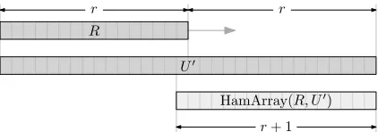
First we introduce an auxiliary stringRof lengthΘ(q3/2). We will user= (q/2)3/2as a shorthand for the length ofR. We will give the details ofRlater but will highlight an important property of it below. We obtainF fromKnby first replacing each 0 by a symbol that we denote?. The symbol?will never occur
in the stream, hence will always generate a mismatch. We then replace every length-rsubstring starting at a 1 with a copy ofR. Any 1 that is closer thanrpositions from the right-hand end ofFis replaced by a
? ? ?
? ? ? ? ? ? ? ? ? ? ? ? ? ? ? ? ? ? ? ? ? ? ? ? ? ? ? ? ? ? ? ? ? ? ? ? ? ? ? ? ? ? ? ? ? ? ? ?
? ? ? R ?? ?
2i
R
n
F
i
Figure 4: The stringFhas a copy ofRstarting at each positionn−1−iwherei≥ |R|is a power of two. All other positions have the symbol?which only occurs inFand not in the stream.
r r
r+ 1 R
U0
(R, U0)
HamArray
Figure 5: HamArray(R,U0)contains the Hamming distances betweenRand every length-rsubstring of U0asRslides alongU0.
6.3 Properties of the stringRand Hamming arrays
The stringRwill play the same role as the value 1 inKn did for the convolution problem, namely it
will allow us to uniquely determine symbols fromU. To see how, we first introduce the notion of a Hamming array, illustrated inFigure 5. For a stringU0 of length 2r, we write HamArray(R,U0)to denote the length-(r+1)array such that fori∈[r+1], HamArray(R,U0)[i]is the Hamming distance between RandU0[i,i+r−1]. That is, HamArray(R,U0)contains the Hamming distances betweenRand every length-rsubstring ofU0.
To see the resemblance with a 1 inKn, we give the following lemma. The proof is non-trivial and
deferred toSection 7.3. A high-level explanation of the lemma is given immediately after its statement.
Lemma 6.1. There exists a constant k>0such that for any r there is a length-r string R∈[q]rwhere q=2r2/3such that
HamArray(R,U0) | U0∈[q]2r ≥qkr.
The lemma says that there is a stringRsuch that over all possibleU0of length 2|R|, one can obtain qΘ(r)distinct Hamming arrays. Since there are onlyq2r possible values ofU0, this means that a
non-negligible fraction of allU0can be put in one-to-one correspondence with Hamming arrays. Thus, as symbols inUv slide past anRin a similar fashion to symbols inUv sliding past a 1 inKn in the hard
distribution for the convolution problem, we can infer a substantial portion of the symbols ofUvfrom the
output symbolsAv, hence obtain large entropy. We formalise this in the next section and explain how the
lower bound is obtained.
6.4 The hard distribution and obtaining the lower bound
`v
1 4`v
1 2`v
F R R R
U0
1 U20 U30 Um0
U0
1 U20 U30 Um0
1
2
3 · · · ·
· · ·
U0
1 U20 U30 · · · Um0
? ? ?· · · ·? ??
· · ·? ??
? ? ? ?· · · ·? ?? ? ?· · · ·?
Figure 6: Three alignments ofF and the streamS:1 the last value ofUv has just arrived,2 half of the
outputs inAvhave been outputted, and3 all outputs inAv have been outputted. The stringUvis here the
concatenation ofU10, . . . ,Um0 ∈UR, wherem=`v/(4r).
Given a stringR∈[q]r, we letU
R⊆[q]2rbe any largest set of length-(2r)strings such that for any
two distinct stringsU10,U20 ∈UR,
HamArray(R,U10)=6 HamArray(R,U20).
To uniquely specify a string inUR we need log2|UR|bits. ByLemma 6.1we have that there exists anR
such that log2|UR| ∈Θ(rlogq).
For the hard distribution we useF from above with anRthat has the properties ofLemma 6.1. The inputU is given by concatenatingn/2rstrings drawn independently and uniformly at random fromUR.
Similarly toFigure 2we can now illustrate how strings from UR slide pastRduring the second
half of the output symbols inAv, wherevis any node ofTsuch that`v≥h·√n. Herehis the positive
constant fromLemma 3.7. We defer picking the value ofhuntil later. For any such node, we have that
`v>h·r because we assumed thatn≥q3and the definition ofr implies thatq3>r2. InFigure 6we have illustratedUvas the concatenation of random stringsU10, . . . ,Um0 drawn fromUR, wherem=`v/(4r).
Between alignments2 and3 in the figure, the second half of the substringsUi0ofUvslide in turn pastR,
and from the outputs inAvwe can infer HamArray(R,Ui0)for each suchUi0. By construction ofUR this
allows us to uniquely determine the stringsUi0. Thus, over all outputsAv, a total of approximatelym/2
substringsUi0ofUv can be completely determined. We pick abovehto be sufficiently large so that, even
compensating for border cases, the number of substringsUi0ofUvthat can be determined is always at least
one. This implies that the entropy ofAvmust, byLemma 6.1, be at leastΘ((m/2)·rlogq) =Θ(`v·δ),
whereδ =dlog2qe. This concludes the proof ofLemma 3.7.
7
A string with many different Hamming arrays
In this section we proveLemma 6.1, that is we show that there exists a stringRwhich gives many different Hamming arrays. This is arguably the most technically detailed part of our lower bound proofs. To recap, we claim that for anyrthere exists a string R∈[q]rwithq=2r2/3which permits at leastqkrdistinct
Hamming arrays when combined with every string in[q]2r, wherekis a constant. Next we describe the
R
µ2−1 | {z }
ρ0
?0? ?0? ?1?1 2? ?2 2 3?3? ? ? ?4? ???5 5?66?6 6?7?7 7?8?8? ? ? ?
| {z }
ρ1
| {z }
ρ2
| {z }
ρ3
| {z }
ρ4
| {z }
ρ5
| {z }
ρ6
| {z }
ρ7
| {z }
ρ8
| {z }
ρ(µ2−1) · · ·
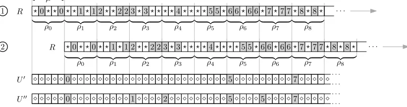
Figure 7: An example of the stringRof lengthr=µ3, which is the concatenation of the µ2 strings ρ0, . . . ,ρµ2−1, whereρi∈ {?,i}µ.
U0
R
| {z }
ρ0
?0? ?0? ?1?1 2? ?2 2 3?3? ? ? ?4? ???5 5?66?6 6?7?7 7?8?8?
| {z }
ρ1 | {z }ρ2 | {z }ρ3 | {z }ρ4 | {z }ρ5 | {z }ρ6 | {z }ρ7 | {z }ρ8 · · ·
R
| {z }
ρ0
?0? ?0? ?1?1 2? ?2 2 3?3? ? ? ?4? ???5 5?66?6 6?7?7 7?8?8?
| {z }
ρ1 | {z }ρ2 | {z }ρ3 | {z }ρ4 | {z }ρ5 | {z }ρ6 | {z }ρ7 | {z }ρ8 · · ·
1
2
µ
0 5 7
U00 0 1 2 5 5 7
Figure 8: Setting symbols ofU0renders a large set of possible Hamming distance outputs.
7.1 The structure ofR
To shorten notation it will be convenient to introduce the variableµ as a shorthand forr1/3. HenceRhas lengthr=µ3andq=2µ2. The stringRis constructed by concatenatingµ2substrings, each of lengthµ.
Fori∈[µ2]we letρi denote thei-th substring ofR, that is
R =ρ0ρ1···ρ(µ2−1).
Each substringρican only contain symbols from the set{?,i}, where?is the special symbol that will not
occur in the stream. Therefore, the total number of distinct symbols inRis at mostµ2+1≤qas claimed.
Figure 7illustrates an example ofR.
The purpose of the substringsρiis to support a reduction from vector addition to Hamming arrays
that we explain next.
7.2 Vector sums and Hamming arrays
Before we describe the full reduction in the following section we begin by giving some high level intuition. We first introduce some notation. LetV ={v0,v1,v2. . .vµ2−1}be a multi-set of vectors where vi∈ {0,1}µ. We can define a correspondence between the length-µ substringρiofRand thei-th vector vias follows. The j-th symbol ofρiequalsiif the j-th component ofviis 1 and?otherwise. For example,
ρ2=2??22 fromFigure 7corresponds to the vectorv2= (1,0,0,1,1).
We will now see that this correspondence between vectors inV and substrings ofRcan be used to encode elementwisesumsof vectors inV in the Hamming array forR. Consider the stringU0∈[q]2r
respectively. The positions holding these symbols are chosen such that in the first alignment betweenR andU0, marked1, the symbols 0, 5 and 7 sit immediately afterρ0,ρ5andρ7inR, respectively. AsR slidesµ steps to the right towards the alignment marked2, the symbols 0, 5 and 7 ofU0will generate matches whenever they are aligned with their corresponding symbols inR. Thus, fori∈ {1, . . . ,µ},
HamArray(R,U0)[i] = r−(v0+v5+v7)[i],
where(v0+v5+v7)[i]is thei-th component of the sum of the vectorsv0,v5andv7. In other words, from HamArray(R,U0)[1,µ]we can uniquely determine the sumv0+v5+v7. As shorthand we will think of HamArray(R,U0)[1,µ]asencodingthe sumv0+v5+v7.
The idea above can be repeated by populatingU0with more symbols from[µ2]. As an example we
have added the symbols 1 and 2, and another copy of 5 toU0, which is the string denotedU00in the figure. AsRslides anotherµ steps to the right, HamArray(R,U00)[µ+1,2µ]encodes (uniquely specifies) the
sumv1+v2+v5.
Observe that as we populateU0with symbols, positions becomeblocked. For example, we could not have added symbols toU0 to define an alternateU00which instead encodes the sumv1+v2+v4in HamArray(R,U00)[µ+1,2µ]since the position where the 4 would have to be set is already occupied
by a 5. Observe however that setting symbols ofU00as above generates matches only in the intended length-µ window of the Hamming array. Thus, we have full control of which vector sums we want to
encode, under the constraint that positions become blocked, limiting the choice of vectors.
The conclusion thus far is that vector sums have a direct correspondence with the Hamming array. Next we take the ideas from above further and show that if there exists a pool ofµ2vectors such that
many different vector sums can be obtained when addingµ vectors from the pool, then the number of
distinct HamArray(R,U0)one can obtain is large. This would proveLemma 6.1.
7.3 The stringRand the proof ofLemma 6.1
Before we state the next lemma which will be used to proveLemma 6.1, we introduce some basic notation that we will use when reasoning about multisets of vectors. LetX be a multiset of vectors. Consider an arbitrary ordering of the elements of X and refer to X[i]as the i-th element ofX. We use the term sub-multiset of X to denote any multiset obtained from X by removing zero or more elements. We will use the notationvto denote the sub-multiset relation so that we have, for example,
{1,1,4,5,5} v {1,1,1,4,4,5,5,7,8}. We can now introduce the required lemma.
Lemma 7.1. For anyµ >40such thatµ−1is a prime, there exists a multiset V of vectors from{0,1}µ
such that|V|=µ(µ−1)and for any sub-multiset V0⊆V of size at least(63/64)|V|,
{w1+···+wµ | {w1, . . . ,wµ} vV0} ≥ µ(µ/10).
Suppose thatV ={v0, . . . ,vµ(µ−1)}is a multiset of length-µ vectors over{0,1}with the properties
ofLemma 7.1. That is, we assume thatµ >40 andµ−1 is a prime. Again as discussed inSection 6.1,
we can always tweak relevant values in order to meet this criteria.
The stringRis simply chosen such that fori∈[µ(µ−1)], the substringρicorresponds to the vectorvi
ofV as described at the start ofSection 7.2. Fori∈ {µ(µ−1), . . . ,(µ2−1)}, the substringρi={?}µ as
we will ignore these substrings anyway. In order to show that thisRprovesLemma 6.1we will populate a length-(2r)vectorU0with symbols and show how length-µ subarrays of HamArray(R,U0)correspond
to vector sums ofµ vectors chosen arbitrarily from a sub-multiset ofV. The process for constructing a stringU0 is as follows:
1. Set all 2µ3positions ofU0to the symbol.
2. AlignRwith the left half ofU0as illustrated inFigure 5.
3. LetV0⊆V be the set of vectors that are not blocked. Initially this means thatV0=V but as we return to this step,V0shrinks.
4. Choose any sub-multiset{w1, . . . ,wµ} vV0and set their corresponding positions inU0accordingly. For anyvi∈ {w1, . . . ,wµ}the corresponding position inU0is the one which is currently aligned with the position immediately after substringpi inR. This position is set to the symboli.
5. SlideRbyµsteps alongU0. Over these alignments, HamArray(R,U0)uniquely specifies the vector
sumw1+···+wµ.
Steps 3–5 are referred to as around.
6. Repeat from Step 3 for a total of (µ−1)/64 rounds. Observe that a total ofµ(µ−1)/64= (1/64)|V|vectors become blocked, hence|V0|is always at least(63/64)|V|.
7. SlideRbyone single stepalongU0. This will offset all previously blocked vectors and allow us to start over again at Step 3 as if no vectors are blocked. This is repeated until this step is reached for theµ-th time. At that point the offsetting of blocked vectors has cycled and previously set positions
ofU0are yet again blocked.
PopulatingU0 according to the procedure above means thatRis shifted by a total of
µ·(µ−1)/64·µ+ (µ−1) = µ3/64−µ2/64+µ−1 < r
steps. Over these steps we have byLemma 7.1that for each length-µ subarray of HamArray(R,U0)that corresponds to a vector sum, there is a choice of at leastµ(µ/10)distinct values. Thus, whenµ >40, the
number of distinct HamArray(R,U0)is at least
µ(µ/10)
µ(µ−1)/64
= µ(µ
3−µ2)/640
≥ µ(µ
3/656)
= r(1/3) (r/656)
= rkr,
8
Vector sets with many distinct sums
In this section, we proveLemma 7.1. We first rephrase the lemma slightly by introducing some notation. For any multisetV0of vectors from{0,1}µ, we define
Sum(V0) ={w1+···+wµ | {w1, . . . ,wµ} vV0}
to be the size of the set of distinct vector sums one can obtain by summing the vectors of size-µ
sub-multisets ofV0. Addition is elementwise and over the integers. Lemma 7.1says that there exists a multiset V of vectors from{0,1}µ such that |V|=µ(µ−1) and for any sub-multisetV0 vV of size at least (63/64)|V|, we have that Sum(V0)≥µ(µ/10).
Our approach will be an application of the probabilistic method. Specifically, we will show that when the vectors ofV are chosen independently and uniformly at random from{0,1}µ, the expected value,
E[Sum(V)] ≥ 1
2(µ−1)
(µ/9).
Thus, there must exist aV such that Sum(V)≥(µ−1)(µ/9)/2. Given such aV, we then show that for every sub-multisetV0vV such that|V0| ≥(63/64)|V|, Sum(V0)≥µ(µ/10).
8.1 Vectors and codes
We now describe a connection between vectors and codes which we will use in our analysis to lower bound the number of distinct vector sums, Sum(V)that can be obtained from a vector setV. We will require the following lemma from the field of Coding Theory. The lemma is tailored for our needs and is a special case of “Construction II” in [1]. For our purposes, a binary constant-weight constant-weight binary cyclic code can be seen simply as set of bit strings (codewords) with two additional properties: the first is that all codewords have constant Hamming weightµ, i. e., they have exactlyµ1s, and the second
property is that any cyclic shift of a codeword is also a codeword.
Lemma 8.1([1]). For any µ ≥4such that µ−1is a prime and any odd γ∈[µ], there is a binary
constant-weight constant-weight binary cyclic code with(µ−1)γ codewords of lengthµ(µ−1)and Hamming weightµ such that any two codewords have Hamming distance at least2(µ−γ).
LetCebe the binary code that containsallcodewords of lengthµ(µ−1)with Hamming weightµ. We can think of a codeword ofCerepresenting a size-µ sub-multisetXvV such that thei-th vector ofV
(under any enumeration of the elements ofV) is inXif and only if positioniof the codeword is 1. That is,Cerepresents all possible sub-multisets ofV of sizeµ. To shorten notation, we refer toec∈Ceas both a codeword and a sub-multiset ofµ vectors fromV.
Suppose thatµ ≥4 andµ−1 is a prime. We letC⊆Cebe a cyclic code of size(µ−1)γ, whereγ is
any odd integer in the interval[µ/9,µ/8], such that the Hamming distance between any two codewords
inCis at least 7µ/4. The existence of such aCis guaranteed byLemma 8.1since 2(µ−µ/8) =7µ/4.
Forc∈Cwe define theball, Ball(c)to be the set of bit strings inCeat Hamming distance at most
µ/16 fromc. Formally,
Ball(c) ={ec | ce∈Ceand Hamming distance betweencandecis at mostµ/16}.
Observe that the|C|balls are all disjoint since the Hamming distance between any two codewords in Cis at least than 7µ/4. In particular, for anyc∈C, Ball(c)∩C={c}. We have that for anyc∈C, using the fact ab≤(ae/b)b,
Ball(c) ≤
µ µ/16
·
|V|
µ/16
≤
µe· |V|e (µ/16)2
µ/16
≤µ
16 µ/16
.
Forec∈Cewe write sum(ce)to denote the vector in[µ+1]µ obtained by adding theµ vectors in the
vector setec, that is sum(ec)vector sum of the vectors represented byec.
Towards provingLemma 7.1we will show that when the vectors ofV are chosen uniformly at random, we expect more than half of all|C|balls to have the property that for everycein the ball, sum(ec)can only be obtained by summing vectors from that ball.
8.2 Choosing the vectors inV
So far we have not discussed the choice of vectors inV. Initially we consider choosing the vectors independently and uniformly at random from{0,1}µ. We will first show that
E[Sum(V)] ≥ 1
2(µ−1)
(µ/9),
then we will fixV and show that this fixedV has the property ofLemma 7.1.
Consider any two distinct c1,c2 ∈C and the corresponding balls, Ball(c1) and Ball(c2) which are disjoint subsets ofCe. For any ce1∈Ball(c1) and ce2∈Ball(c2), we now analyse the probability that sum(ce1) =sum(ce2). From the definitions above it follows thatce1 and ce2 must differ on at least 7µ/4−2(µ/16)≥µ positions, implying that the two vector setsce1andce2have at mostµ/2 vectors in
common, thus at leastµ/2 of the vectors ince1are not ince2. Letw1, . . . ,w(µ/2)denote an arbitrary choice
ofµ/2 of those vectors. Fori∈[µ]we can write thei-th component of sum(ce1)as
sum(ce1)[i] = w1[i] +···+w(µ/2)[i] +x[i],
where the vectorxdoes not depend onw1, . . . ,w(µ/2). In order to have sum(ce1) =sum(ce2)we must have w1[i] +···+w(µ/2)[i] = sum(ce2)[i]−x[i]
for eachi∈[µ]. Since the vectors are picked independently and uniformly at random from{0,1}µ, the
most likely value ofw1[i] +···+w(µ/2)[i]isµ/4. The probability that this sum equalsµ/4 is
Pr
w1[i] +···+w(µ/2)[i] =
π
4
=
µ/2 µ/4
·
1 2
µ/2
≤ µ
2 −1/2

![Figure 3: An illustration of A = U ×F. Digits of U arrive one at a time, where U[0] is the low-order digitthat arrives first.](https://thumb-us.123doks.com/thumbv2/123dok_us/8363392.1672453/16.612.103.513.108.252/figure-illustration-digits-arrive-order-digitthat-arrives-rst.webp)