1499 IJSTR©2019
Optimization Of Surface Roughness Using Jaya
Algorithm In EDM
Neeraj Agarwal, Dr. Nitin Shrivastava, Dr. M. K. Pradhan
Abstract: Electric discharge machining (EDM) is the most popular advanced machining process. EDM is able to cut any material. Titanium alloy has very good strength to weight ratio but It is very difficult to cut with conventional machining processes. Finishing process required an excellent surface finish. In this research paper surface roughness (Ra) is optimized. Four input parameter peak current (Ip), pulse on time (Ton), duty factor (t) and voltage (V) considered as a process control parameter. Response surface methodology is used to develop a predictable mathematical model to show the relation between surface roughness and four input parameter Ip, Ton, t, and V. This mathematical model is used to optimize surface roughness using advanced optimization technique – Jaya algorithm.
Index Terms: EDM, electric discharge machining, surface roughness, optimization, Jaya algorithm, advanced optimization, single objective optimization, RSM, Titanium alloy.
—————————— ——————————
1.
INTRODUCTION
ELECTRICAL discharge machining (EDM) is used to machine difficult to cut material. Two electrodes (workpiece and tool) is kept at a certain distance known as electrode gap. Both electrodes are submerged in dielectric fluid and voltage is applied between electrodes. As soon as breakdown voltage achieved sudden sparking takes place between electrodes [1]. Due to this sparking a very high local temperature is achieved at machining area and some material is melt and evaporated material from workpiece and tool [2]. A mathematical model shows the relation between input variables and quality measures (output). This model is used for optimization. Some time it is very difficult to optimize with convectional optimization techniques If numbers of input parameter increases or mathematical modeling are more complex. To overcome this limitation advanced optimization is more popular nowadays [3]. With the increasing use of computer population-based metaheuristic like evolutionary algorithm based optimization like a genetic algorithm (GA) [4], Evolutionary Programming (EP). Some optimization technique based on nature-inspired like particle swarm optimization (PSO), firefly algorithm. Particle swarm optimization requires some algorithm-specific parameter and this requires constant tuning of these parameters. A high-speed computer is required to solve this optimization problem [5]. To overcome this algorithm-specific parameter Rao introduce a new optimization technique known as Teaching–learning-based optimization (TLBO) [6]. TLBO does not require any algorithm-specific parameter. In 2016 new advanced optimization technique introduced by Rao is known as Jaya algorithm [7,8]. Jaya algorithm is efficient and powerful optimization technique and being more popular nowadays.
Das et al. used an artificial bee colony to optimize surface roughness (Ra) [9]. Manjaiah et al. reviewed on machining of titanium alloy [10]. Agarwal et al. used Jaya algorithm to optimized EDM process parameter [11]. Shrivastava et al. used artificial neural network-based modeling followed by optimization with a genetic algorithm [12]. In this research paper response surface methodology used to develop a mathematical model which is followed by optimization using Jaya algorithm.
2
EXPERIMENTAL
SETUP
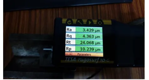
Titanium alloy is selected as the workpiece. Workpiece size is 50X50X5 mm. 10 mm diameter copper rod is selected as the workpiece. Current (Ip), Voltage (V), pulse on time (Ton) and duty factor (t) is selected as a process parameter. Response surface methodology (RSM) is selected for the design of experiments (DOE). Three-level of the parameter is selected as per table 1. Thirty experiments were conducted as per DOE on electronica S50 CNC electric discharge machining. Each experiment were conducted for 30 minutes. After experiments surface roughness were measured using surface profilometer ―TESA-rugosurf 10-G‖ make as shown in figure 1. Table 2 shows the experimental observation of Ra
————————————————
Neeraj Agarwal is currently pursuing PhD degree program in University Institute of Technology, RGPV, Bhopal, India, PH-+919926383834. E-mail: [email protected]
Dr. Nitin Shrivastava is currently working as Associate Professor at department of Mechanical Engineering, University Institute of Technology, RGPV, Bhopal, India. E-mail: [email protected]
Dr. M. K. Pradhan is currently working as Assistant Professor at department of Mechanical Engineering, Maulana Azad National Institute of Technology (MANIT), Bhopal, India. E-mail: [email protected]
Table 1: Process control parameters and range Parameter Level 1 Level 2 Level 3
Ip (A) 4 6 8
V (Volt) 40 70 100
Ton (µs) 50 100 150
t(duty factor) 8 12 16
Table 2: Experimental observation of Ra Exp.
Ip V Ton t Ra
1 8 40 150 50.0 5.134
2 8 40 50 25.0 3.152
3 4 40 50 25.0 2.952
4 8 40 50 50.0 5.294
5 6 70 100 37.5 3.784
6 6 70 100 37.5 3.815
7 6 70 100 37.5 3.746
8 4 40 50 50.0 3.267
9 4 40 150 50.0 4.202
10 4 100 150 25.0 3.954
11 4 40 150 25.0 4.468
12 4 100 50 50.0 4.138
13 4 100 50 25.0 3.274
14 8 100 50 50.0 6.637
15 6 70 100 37.5 3.812
16 8 100 150 50.0 5.260
17 8 100 150 25.0 4.480
18 8 40 150 25.0 3.993
19 4 100 150 50.0 3.880
20 8 100 50 25.0 4.267
21 6 70 50 37.5 3.581
22 6 40 100 37.5 3.716
23 6 100 100 37.5 4.092
24 6 70 100 50.0 4.334
25 6 70 100 25.0 3.543
26 6 70 100 37.5 3.727
27 6 70 150 37.5 3.632
28 8 70 100 37.5 4.129
29 6 70 100 37.5 3.872
30 4 70 100 37.5 3.506
Modeling: A regression model is developed using commercial software Minitab 18 as following. Response surface methodology (RSM) methodology is used.
Ra=4.390 - 0.2707 Ip - 0.0313 V + 0.04200 Ton - 0.1395 t + 0.000268 V*V+ 0.001767 t*t + 0.002826 Ip*V 0.002097 Ip*Ton + 0.01398 Ip*t- 0.000161 V*Ton 0.000411 Ton*t (1)
3 JAYA
ALGORITHM
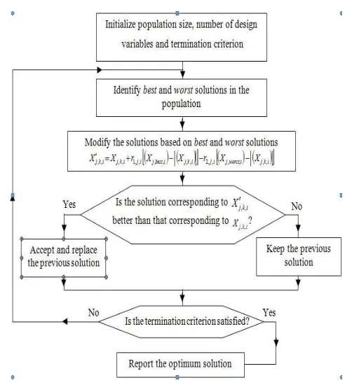
Jaya algorithm is an advanced optimization algorithm used in engineering optimization. Jaya algorithm works on iteration and with each iteration, it moves toward the best solution and moves away from worst solution simultaneously. Figure 2 shows flow diagram of Jaya Algorithm.
New value of variable modified as per following equation
X'j,k,i = Xj,k,i + r1,j,i (Xj,best,i - │Xj,k,i│) - r2,j,i (Xj,worst,i - │Xj,k,i│) (2)
Where X'j,k,i is new value of variable, i=iteration number, Xj,k,i is the value of the jth variable for the kth candidate during the I th iteration, r1 and r2 is random numbers within the range [0, 1]. Xj,best,i is best candidate value and Xj,worst,i worst candidate value.
4 ADVANCED
OPTIMIZATION
USING
JAYA
ALGORITHM
Jaya algorithm used to solve the optimization problem on surface roughness (Ra)
Step 1: Initial population: Initial population is random numbers of variables within the range of variables as specified in table 1.
Table 3: Initial solution /population Ca
n. Ip Ton t V Ra
Rem ark 1 7.3244 142.8011 29.2371 93.0242 4.1155 2 5.5515 124.1502 29.3529 91.2023 3.8467 3 5.5303 94.7873 31.1149 63.8871 3.4561 Best 4 5.0858 120.9639 41.0232 46.9296 3.8137 5
7.4715 144.4331 45.2153 44.8169 4.5541 Wors t
Step 2: Objective function equation (1) is calculated for each candidate and written in table 3 under column Ra. The objective is to minimize surface roughness (Ra) hence the minimum value of surface roughness (Ra) is marked as best while the maximum value of Ra is marked as worst. In table 3
1501 IJSTR©2019
candidate 3 is marked as best and candidate 5 marked as worst. Under third candidate Ip_best=5.5303, Ton_best=94.7873, t_best=31.1149 and V_best=63.8871. Under fifth candidate Ip_worst=7.4715, Ton_worst=144.4331, t_worst=45.2153 and V_worst=44.8169. Consider two random numbers r1=0.3605 and r2=0.8289 within the range of 0 and 1.
Step 3: As per equation 2, new values of variables are calculated and inserted into table 4.
X'j,k,i = Xj,k,i + r1,j,i (Xj,best,i - │Xj,k,i│) - r2,j,i (Xj,worst,i - │Xj,k,i│) (2)
Ip1= 7.3244+ 0.3605*(5.5303-|7.3244|)- 0.8289*(7.4715-|7.3244|) = 6.5556
Ip2= 5.5515+ 0.3605*(5.5303-|5.5515|)- 0.8289*(7.4715-|5.5515|) = 3.9523 (=4 because lower bound of Ip value is 4 as per table 1)
Ip3= 5.5303+ 0.3605*(5.5303-|5.5303|)- 0.8289*(7.4715-|5.5303|) = 3.9212 (=4 because lower bound of Ip value is 4 as per table 1)
Ip4= 5.0858+ 0.3605*(5.5303-|5.0858|)- 0.8289*(7.4715-|5.0858|) = 3.2685 (=4 because lower bound of Ip value is 4 as per table 1)
Ip5= 7.4715+ 0.3605*(5.5303-|7.4715|)- 0.8289*(7.4715-|7.4715|) = 6.7716
Ton1= 142.8011+0.3605*(94.7873-|142.8011|)-0.8289*(144.4331-142.8011|) = 124.1393603
Ton2= 124.1502+0.3605*(94.7873-|124.1502|)-0.8289*(144.4331-124.1502|)= 96.75237874
Ton3= 94.7873+ 0.3605*(94.7873-|94.7873|)-0.8289*(144.4331-|94.7873|)=53.63589638
Ton4= 120.9639+ 0.3605*(94.7873-|120.9639|)- 0.8289*(144.4331-120.9639|)=92.07361582
Ton5= 144.4331+ 0.3605*(94.7873-|144.4331|)-0.8289*(144.4331-144.4331|)= 126.5357891
t1= 29.2371+ 0.3605*(31.1149-|29.2371|)- 0.8289*(45.2153-|29.2371|) =16.6697 (=25 because lower bound of ―t‖ value is 25 as per table 1)
t2= 29.3529+ 0.3605*(31.1149-|29.3529|) -0.8289*(45.2153-|29.3529|) =16.8397 (=25 because lower bound of ―t‖ value is 25 as per table 1)
t3= 31.1149+ 0.3605*(31.1149-|31.1149|) -0.8289*(45.2153-|31.1149|)= 19.4270 (=25 because lower bound of ―t‖ value is 25 as per table 1)
t4= 41.0232+ 0.3605*(31.1149-|41.0232|) -0.8289*(45.2153-|41.0232|)=33.9764
t5= 45.2153+ 0.3605*(31.1149-|45.2153|) -0.8289*(45.2153-|45.2153|)= 40.1321
V1= 93.0242+ 0.3605*(63.8871-|93.0242|) -0.8289*(44.8169-|93.0242|)= 122.4793064 (=100 because upper bound of ―V‖ value is 100 as per table 1)
V2= 91.2023+ 0.3605*(63.8871-|91.2023|) -0.8289*(44.8169-|91.2023|)= 119.8040285 (=100 because upper bound of ―V‖ value is 100 as per table 1)
V3= 63.8871+ 0.3605*(63.8871-|63.8871|) -0.8289*(44.8169-|63.8871|)= 79.69438878
V4=46.9296+ 0.3605*(63.8871-|46.9296|) -0.8289*(44.8169-|46.9296|)= 54.79399578
V5= 44.8169+ 0.3605*(63.8871-|44.8169|) -0.8289*(44.8169-|44.8169|)= 51.6917071
Table 4: New values of variables and corresponding objective function value (during the first iteration).
Candidate Ip Ton t V Ra
1 6.5558 124.1409 25 100 4.1592
2 4 96.7533 25 100 3.7027
3 4 53.6355 25 79.6945 2.9941
4 4 92.0743 33.9768 54.7935 3.213 5 6.7718 126.5374 40.1326 51.691 4.0685
Step 4: Now compare table 3 and table 4 for each candidate. Candidate 1 has a value of Ra in table 3 has 4.1155 while candidate 1 from table 4 has Ra value is 4.1592. The objective is to minimize Ra hence candidate 1 from table 3 has better value hence select candidate 1 from table 3 and insert into table 5. Similar candidate 2, 3, 4 and 5 of Table 4 has better value as compared to table 3 hence select candidate 2,3,4 and 5 from table 4 and insert into table 5.
Table 5: Updated values of variables and corresponding objective function (during the first iteration).
Can
. Ip Ton t V Ra
1
7.3244 142.8011 29.2371 93.0242 4.1155
From table 3 2
4 96.7533 25 100 3.7027
From table 4 3
4 53.6355 25 79.6945 2.9941
From table 4 4
4 92.0743 33.9768 54.7935 3.213
From table 4 5
6.7718 126.5374 40.1326 51.691 4.0685
From table 4
Step 5: Iteration 1 is over. Table 5 would be input for the next iteration (same as table 3).
Step 6: Consider random numbers r1=0.2146 and r2=0.7910 for second iteration. Repeat the same procedure from step 1 to step 4.
Table 6: New values of variables and corresponding objective function (for the second iteration)
Candidate
Ip Ton t V Ra
1 6.611 123.6653 28.3278 90.1635 3.9704 2
4 51.0741 25 100 3.3721
3 4 50 25 69.1501 2.831
4
4 50 35.7995 40 2.8316
Table 7: Updated values of the variable for the second
iteration
Step 7: Repeat the iteration to certain numbers of time like 100 or any numbers as per requirement.
Table 8: Best solution iteration wise.
Iteration Ip Ton t V Ra
1 5.5303 94.7873 31.1149 63.8871 3.4561
2 4 53.6355 25 79.6945 2.9941
3 4 50 25 69.1501 2.831
4 4 50 28.6159 58.7785 2.7324
5 4 50 27.0659 53.378 2.7304
6 4 50 27.0659 53.378 2.7304
7 4 50 28.864 55.0363 2.7226
8 4 50 29.6703 49.6234 2.722
9 4 50 29.6703 49.6234 2.722
10 4 50 29.2314 51.475 2.7202
11 4 50 29.2314 51.475 2.7202
12 4 50 29.2314 51.475 2.7202
13 4 50 29.2314 51.475 2.7202
14 4 50 29.2314 51.475 2.7202
15 4 50 29.2314 51.475 2.7202
16 4 50 29.2314 51.475 2.7202
17 4 50 29.1503 51.9951 2.7202
18 4 50 29.1503 51.9951 2.7202
19 4 50 29.1503 51.9951 2.7202
20 4 50 29.1503 51.9951 2.7202
21 4 50 29.1682 52.1076 2.7201
22 4 50 29.1682 52.1076 2.7201
23 4 50 29.1682 52.1076 2.7201
24 4 50 29.169 52.1126 2.7201
25 4 50 29.2305 51.988 2.7201
26 4 50 29.2305 51.988 2.7201
27 4 50 29.2435 51.9637 2.7201
28 4 50 29.2272 52.1769 2.7201
29 4 50 29.2792 52.2615 2.72
30 4 50 29.3714 52.4118 2.72
31 4 50 29.3714 52.4118 2.72
32 4 50 29.4719 52.4989 2.72
33 4 50 29.4719 52.4989 2.72
34 4 50 29.4717 52.4545 2.72
35 4 50 29.5454 52.1212 2.7199
100 4 50 29.5454 52.1212 2.7199
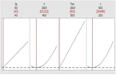
Figure 4: Optimization plot
Table 8 shows iteration wise best result. Figure 3 shows the convergence graph of Ra and figure 4 shows the effect of various parameter on surface roughness.
5 CONCLUSIONS
Surface roughness (Ra) is successfully optimized using Jaya algorithm. To optimize surface roughness peak current (Ip) and pulse on time (Ton) should have minimum value where Ip=4 A, Ton= 50 µs. Duty factor (t) should be 29.5455 %, voltage (V) have 52.1212 and minimum surface roughness (Ra) achieved 2.7199 µm. Jaya algorithm took only 35 iterations to achieve the optimum solution. Jaya algorithm is suitable for an engineering optimization problem.
REFERENCES
[1] Jain, Vijay Kumar. Advanced machining processes. Allied publishers, 2009.
[2] Ho, K. H., and S. T. Newman. "State of the art electrical discharge machining (EDM)." International Journal of Machine Tools and Manufacture 43.13 (2003): 1287-1300. [3] Rao, R. Venkata, and V. D. Kalyankar. "Optimization of modern machining processes using advanced optimization techniques: a review." The International Journal of Advanced Manufacturing Technology 73.5-8 (2014): 1159-1188.
[4] Deb, Kalyanmoy, et al. "A fast and elitist multiobjective genetic algorithm: NSGA-II." IEEE transactions on evolutionary computation 6.2 (2002): 182-197.
[5] Kennedy, James. "Particle swarm optimization." Encyclopedia of machine learning (2010): 760-766.
[6] Rao, R. Venkata, Vimal J. Savsani, and D. P. Vakharia. "Teaching–learning-based optimization: a novel method for constrained mechanical design optimization problems." Computer-Aided Design 43.3 (2011): 303-315. [7] Rao, R. "Jaya: A simple and new optimization algorithm
for solving constrained and unconstrained optimization problems." International Journal of Industrial Engineering Computations 7.1 (2016): 19-34.
[8] Rao, Ravipudi Venkata. Jaya: an advanced optimization algorithm and its engineering applications. Cham: Springer International Publishing, 2019.
[9] Das, Milan Kumar, et al. "Application of artificial bee colony algorithm for optimization of MRR and surface roughness in EDM of EN31 tool steel." Procedia materials
Candidate Ip Ton t V Ra
1 6.611 123.6653 28.3278 90.1635 3.9704 2
4 51.0741 25 100 3.3721
3 4 50 25 69.1501 2.831
4 4 50 35.7995 40 2.8316
5 6.7718 126.5374 40.1326 51.691 4.0685
1503 IJSTR©2019
science 6 (2014): 741-751.
[10]Manjaiah, M., S. Narendranath, and S. Basavarajappa. "A review on machining of titanium based alloys using EDM and WEDM." Rev. Adv. Mater. Sci 36.2 (2014): 89-111. [11]Agarwal, Neeraj, M. K. Pradhan, and Nitin Shrivastava. "A
new multi-response Jaya Algorithm for optimisation of EDM process parameters." Materials Today: Proceedings 5.11 (2018): 23759-23768.