Workspace And Analysis Of Five Axes Manipulator Using Swarm Algorithm

713 IJSTR©2019

Workspace And Analysis Of Five Axes

Manipulator Using Swarm Algorithm

Ashwani K., Vijay K., Darshan K.

Abstract: In this paper, the kinematics solution of five degrees of freedom Pioneer arm with six revolute joints using swarm algorithm has been presented. DH parameters are used to obtain the kinematics analysis of the manipulator. Simulations have been performed on the MATLAB with ANFIS to show the workspace of the robotic manipulator. Firefly algorithms and Grey wolf optimization have been used for the minimization of errors. The errors have been optimized to minimum value at different Iterations.

Index Terms:Anfis, Error, Firefly, Grey wolf, Matlab, Robotic arm, Workspace.

————————————————————

1

I

TODAY’S Robotics is used in industry from entertainment to manufacturing. In the manufacturing, production has been increased with the state of art quality. The industrial manipulators are finding applications in various industries like submarine, plastics, food, agricultural, medical, railways, energy and aerospace [1], [2]. The complexity of the robotic arm depends on the increasing number of degrees of freedom. Different tools can be used in certain cases like Cutting tool, Welding tool, Spray painting toll etc. [5]. In the last four decades, different optimization algorithms have been used to find the inverse kinematics solutions for five and more DOF manipulator by applying analytical or numerical methods [1], [2], [6]. In the 6-DOF robotic arm, location and orientation of the end-effector were determined respectively, with the help of first three joints and the last three joints, which are convenient to control and teaching [7], [8]. For higher degrees of freedom robotic arms, the kinematics solution of polynomials with transcendental variables is required [9], [10]. Soft computing techniques used by the researchers are MATLAB, fuzzy logic, adaptive neuro-fuzzy inference system (ANFIS), genetic algorithm (GA) [6], [9], [17], swarm, and evolutionary algorithms (EA) [11], [14], [15], [19], [24], [26] to optimized results.

2

M

Industrial robots are available in the wide range of robotic arm structures with specific work volume as per their DOF structure [5]. Industrial robots have following configurations: 1. Polar Configuration 2. Cylindrical Configuration 3. Cartesian coordinate 4. Articulated configuration Denavit and Hartenberg have given four general parameters to get the kinematics equations of the different DOF robotic manipulators.

But with the advents in research various approaches has been described. The four parameters di, ai, θi, and αi were known as link offset, link length, joint angle, and link twist respectively [5], [12]. The homogeneous transformation matrix is given by

𝑇 =

   

 

   

 

1 0 0 0

3 2 1

P az sz nz

P ay sy ny

P ax sx nx

(1)

Here n, s, a, and p are the elements of rotation and position matrices for x, y, and z-axis [12]. The transformation matrix A for any angle theta can be written as in (2).

A =

   

 

   

 

 

1 0

0 0

cos sin

0

sin . sin . cos cos . cos sin

cos . cos . sin cos . sin cos

d a a

 

     

 

   

(2)

Ai1

i = A

0 1A

1 2A

2 3 A

3

4 … … … A 1 

n

n (3)

Pioneer Arm (Parm) is part of Pioneer 2- and 3-DX robots. It finds applications in research, because it’s not costly than other robotic arms. The arm has pivoting and rotating joints to firm gripping. The Parm 5-DOF manipulator is shown in fig.1.

Fig. 1. 5-DOF Parm manipulator [16]

_________________________________-

 Ashwani Kumar,Department. of ECE, YCOE, Punjabi University Guru Kashi Campus, Talwandi Sabo, India, E-mail: [email protected]

 Vijay Kumar, Department of ECE, ACET, Amritsar,India

 E-mail: [email protected]

 Darshan Kumar, Department of ME,BCET, Gurdaspur, India,

714

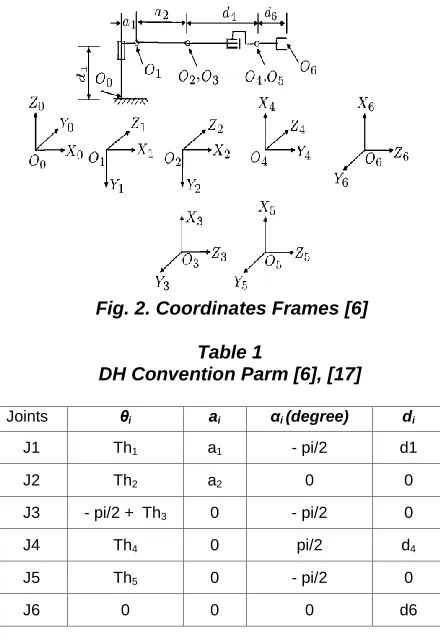
Fig. 2. Coordinates Frames [6]

Table 1

DH Convention Parm [6], [17]

Joints θi ai αi (degree) di

J1 Th1 a1 - pi/2 d1

J2 Th2 a2 0 0

J3 - pi/2 + Th3 0 - pi/2 0

J4 Th4 0 pi/2 d4

J5 Th5 0 - pi/2 0

J6 0 0 0 d6

The joints axis has been assigned using DH representation as written in Table-1 The homogeneous matrices 𝐴 𝑡𝑜 𝐴 can be obtained by substituting the values of parameters of θi, ai, αi and di in (1). Homogeneous matrix 𝐴 can be calculated by multiplying the matrix𝐴 𝑡𝑜 𝐴 . The forward kinematics equations are given by:

P = (−d6c1s23c4c5 + d6s1s4s5 +

d6c1c23c5 + d4c1c23 + a2c1c2 + a1c1); (4)

P = (−d6s1s23c4c5 + d6c1s4s5 +

d6s1c23c5 + d4s1c23 + a2s1c2 + a1s1); (5)

P = (−d6c23c4s5 − d6s23c5 − d4s23 −

a2s2 + d1); (6)

The values of n, s and a for x, y and z has been calculated. Inverse kinematics equations for joint angles Th1 to Th5 can be calculated using matrix inversion method. In this method

 



A _∗ A₁0 = I; (7)

1

A ₌

 

1 5 6  A

(8)

A0₅ T *A1; (9)

Here I is the identity matrix and T from (1) homogeneous matrix. After equating the both sides elements of both matrices has been compared and the joint angles has been calculated. The joint angles have multiple solutions. The angles obtained have particular solution if the end-effector will reach to the desired goal. As the DOFs increases the complexity of the robotic arm structure also increases and it becomes very difficult to find the solution using classical methods.

3

S

The Workspace in XYZ coordinates for the robotic arm with the joint angles range (-365 to 365, -150 to 30, -210 to 60, 0 to 360 and 90 to 60) [2], [6] has been evaluated using MATLAB as shown in fig.3.

Fig. 3. Workspace

The error due to the joint movement from one position to the target position of 5-DOF arm gives rise to change in the set of joint angles to reach to the desired position. The joint angles for the five axes robotic arm with minimum position and absolute error have been calculated using GWO and firefly algorithm. Firefly uses the principle of absorption and attraction of the fireflies [11], [13], [26]. The firefly parameters used are γ, α, β0, and δ known as light absorption coefficient, mutation coefficient, attraction coefficient base value, and uniform mutation range respectively. α_damp is the mutation coefficient damping ratio [11], [13], [25]. Grey Wolf Optimization (GWO) is based on the hunting leadership hierarchy of wolves. Hierarchies exist in pack having α as leader, β, and δ assist α in taking the decision to target prey. ω wolves are followers [9], [15]. The values of these parameters can be considered using different combinations at different iterations. The fitness function is given by

Fitness = l ∗ f + l ∗ f (10) In equation (10) f1 and f2 are the fitness’s for the position error and absolute error. Absolute error is the difference between the predicted and deduced values of joint angles Th1 to Th5. l1 and l2 are the weights. The values of l1 {0 to 1} and l2 {0 to 1} depend on the priority of using functions f1 and f2.

4

R

Considering for the Pioneer arm, the target position (px py pz) at (50, -140, 120) mm and having population size (no. of fireflies) of 40. The values of parameters used are a1=70mm, a2=160mm, d1=130mm, d4=140mm, d6=120mm. The results for the fitness function of (10) and calculated values of f1, f2, X, Y, and Z with joint angles are shown in Table-2, 3 and 4 at different iterations (It).

-40 -20

0 20

40

0 20 40 -20 -10 0 10 20

X0 6

X-Y-Z coordinates generated for all thetas for Parm Robotic arm combinations using forward kinematics formula

Y0₆

Z0

715 IJSTR©2019

0 500 1000 1500 2000 2500

0 5 10 15 20 25 30 35

iteration

fi

tn

e

s

s

Table 2

Iteration and Fitness (f1, f2)

S. No. It f1 f2

1 200 2.41E-01 0.00E+00

2 400 5.91E-03 0.00E+00

3 600 7.67E-05 _3.55E-15

4 800 2.13E-06 2.31E-14

5 1000 4.24E-08 _1.35E-14

Table 3 Iteration and Fitness

S. No. It Fitness Calculated X,Y,Z

1 200 9.63E-02 49.814, -140.0171, 120.1519 2 400 2.36E-03 49.9969, -139.9962,

120.0033 3 600 3.07E-05 50.0000, -140.0000,

119.9999 4 800 8.53E-07 50.0000, -140.0000,

120.0000 5 1000 1.70E-08 50.0000, -140.0000,

120.0000

Table 4

Iteration and Joint angles

S.

No. It Th1 Th2 Th3 Th4 Th5

1 200 -56.86 _20.03 - _34.68 - 114.65 -1.38

2 400 43.56 _66.13 - -9.45 36.31 -5.15

3 600 -8.38

-17.87 -3.31 57.79 -29.78 4 800 74.96 _79.25 - _72.33 - 67.94 7.54

5 100

0 37.32 -71.18

-34.64 70.64 -1.20

The fitness of 1.71E-14 has been obtained at 2500th Iteration and the graph plotted between fitness and Iteration is shown in fig.4.

Fig. 4. Fitness vs. Iteration

When distance will be the only criterion, then f1 becomes the fitness as in (10). The results obtained are shown in Table-5, 6 and 7.

) S.

No. It f1 f2

1 200 3.49E-01 18.849556

2 400 3.85E-03 37.699112

3 600 1.46E-04 100.530965

4 800 1.74E-06 75.398224

5 1000 2.31E-08 62.831853

Table 6

Iteration and Fitness (f1)

S. No. It f1 Calculated X,Y,Z

1 200 2.44E-02 49.7283, _119.8033 -140.0961,

2 400 1.39E-04 49.9999, -139.9962,

120.0006

3 600 8.42E-07 50.0001, _119.9999 -140.0001,

4 800 6.06E-09 50.0000, -140.0000,

120.0000

5 1000 4.94E-11 50.0000, -140.0000,

120.0000

Table 7

Iteration and Joint angles

S.

No. It Th1 Th2 Th3 Th4 Th5

1 200 0.35

-13.00 -28.16

-47.14 111.62 2 400 0.00 23.99 -49.87

-58.43 47.30 3 600 0.00

-50.93 -90.21

-28.82 68.29 4 800 0.00

-58.66 -1.58

-59.76 58.22 5 100

0 0.00 36.90 1.85

-34.79 62.29

The fitness of 5.734E-14 has been obtained at 2500th Iteration and the graph plotted between fitness and Iteration is shown in fig.5.

Fig. 5. Fitness (f1) vs. Iteration

0 500 1000 1500 2000 2500

0 5 10 15 20 25 30 35 40

iteration

fi

tn

e

s

716 When only absolute error is considered f2 will be the fitness

as in (10) then results obtained is shown in Table-8, 9 and 10.

Table 8

Iteration and Fitness (f1, f2)

S. No. _{It f1 f2}

1 200 339.343521 0.00000

2 400 256.723440 0.00000

3 600 228.537699 0.00000

4 800 557.592812 0.00000

5 1000 339.343521 0.00000

Table 9

Iteration and Fitness (f2)

S. No. It f2 Calculated X,Y,Z

1 200 0.00000 44.5009, 192.8424, 54.1234

2 400 0.00000 6.6186, -122.0262, 372.3924 3 600 0.00000 66.6043, -106.3651, _345.4384

4 800 0.00000 -183.252, 236.5464, _458.6976

5 1000 0.00000 44.5009, 192.8424, 54.1234

Table 10

Iteration and Joint angles

S.

No. It Th1 Th2 Th3 Th4 Th5

1 200 8.08

-62.86 -34.91 107.8

1 -14.68 2 400 -7.38

-37.84 -14.46 54.86 0.43 3 600 4.00

-57.54 -7.84 48.70 4.76 4 800 -10.31 24.54 -57.24 78.19 -31.64 5 100

0 8.08

-62.86 -34.91 107.8

1 -14.68

The fitness (f2) shows zero error at 2500th Iteration but due to the change in distance exact target position cannot be obtained as shown in Table-9. The graph plotted between fitness (f2) and Iteration is shown in fig.6.

Fig. 6. Fitness (f2) vs. Iteration

Homogeneous matrix obtained for the 2500th iteration for joint angles at fitness f1 (distance) and f2 (Error) has been obtained. The accurate target position has been achieved.

T =

   

 

   

 

 

 



 



1 0

0 0

000 . 120 277 . 0 543 . 0 793 . 0

00 . 140 953 . 0 263 . 0 153 . 0

000 . 50 126 . 0 798 . 0 590 . 0

(12)

The results obtained at different iterations with different parameters of firefly algorithm shows best results for combinations of fitness f1 and f2 as shown in Table-2, but the individual outputs for fitness f1 and fitness f2 does not show accurate results as can be seen in Table-5 and 8. Comparison graph for the Fitness, f1 (distance) and f2 (Error) has been shown in fig.7.

Fig. 7. Comparison graph between Fitness vs. Iteration for Fitness, f1 (distance) and f2 (Error) (Firefly Algortihm)

To get the results for the GWO, Considering for the Pioneer arm, the target position (px py pz) at (50, -150, 120) and having population size of 50. The results for the fitness function of (10) and values of f1 and f2 are shown in Table-11 and 12 at different iterations (It).

Table 11

Iteration and Fitness (f1, f2)

S. No. _{It f1 f2}

1 200 2.15024 1.11E-15

2 400 2.29126 2.22E-16

3 600 1.36049 0.00000

4 800 2.03431 2.22E-16

5 1000 1.69384 2.22E-16

0 500 1000 1500 2000 2500

0 5 10 15 20 25 30 35

iteration

fi

tn

e

s

717 IJSTR©2019

Table 12 Iteration and Fitness (f)

S. No. _{It f}

1 200 0.40556785

2 400 0.44261751

3 600 0.75042839

4 800 0.44846536

5 1000 0.83431573

The fitness of 2.22E-16 has been obtained for f2 at 1000th Iteration and the graph plotted between fitness and Iteration is shown in fig.8.

Fig. 8. Fitness vs. Iteration (GWO)

From the above results as shown in Table-2 and 3 using Firefly algorithm, shows better fitness for f1 and f2, but for the GWO as in Table-11 and 12 the value of f1 is small as compared to f2. It gives rise to small fitness value using GWO. The results of firefly are comparatively much better than GWO.

5

C

This paper presents the kinematics modeling of 5-DOF robotic arm having six revolute joints using matrix inversion methods to deduce the joint angles for the desired location. The workspace for 5-DOF manipulator has been found using MATLAB and graph between the fitness function and iteration has been obtained using Grey wolf and Firefly algorithm. The results obtained give us accurate target position and reduces the overall errors to almost zero. When the individual errors are considered target position may or may not be achieved. As the number of iterations increases the computation time also increases. The results of Firefly are better than the GWO.

R

[1] A. Patil, M. kulkarni, A. Aswale,―Analysis of the inverse kinematics for 5 DOF robot arm using D-H parameters‖,

Pro. IEEE international conference on real-time

Computing and Robotics, pp. 688-693, 2017.

[2] C. Urrea, J. Kern,―Design, simulation and comparison of controllers for a redundant robot‖, Case Studies in

Mechanical systems and signal Processing, 3 (2016)

9-21.

[3] S.R. Deb,―Robotics technology and flexible automation‖, Tata McGraw Hill, 2002.

[4] R.J. Schilling,―Fundamental of Robotics: Analysis and Control‖, Prentice Hall, India Pvt. Ltd., 2002.

[5] Fu K.S., Gonzalez R.C., Lee C.S.G.,―Robotics: Control, Sensing, Vision and Intelligence‖, McGraw Hill International Editions, 1987.

[6] D. Xu, C.A.A. Calderon, J.Q. Gan, H. Hu, ―An Analysis of the Inverse Kinematics for a 5-DOF Manipulator‖,

International Journal of Automation and Computing 2

(2005) pp.114-124.

[7] M.F. Aly, A.T. Abbas, and S.M. Megahed, ―Robot workspace estimation and base placement optimisation techniques for the conversion of conventional work cells into autonomous flexible manufacturing systems‖,

International Journal of Computer Integrated

Manufacturing 23(12), 2010, pp. 1133–1148.

[8] A. Khatamian,―Solving Kinematics Problems of a 6-DOF Robot Manipulator‖, Proc. Int'l Conf. Scientific Computing (CSC'15), pp. pp. 228-233, 2015.

[9] S. Alavandar, M.J. Nigam,―Neuro-Fuzzy based Approach for Inverse Kinematics Solution of Industrial Robot Manipulators, Int. J. of Computers, Communications &

Control, III (3), 2008, pp.224-234.

[10]M. Dahari, and J. Tan,―Forward and Inverse Kinematics Model for Robotic Welding Process Using KR-16KS KUKA Robot‖, Proc. 2011 Fourth International Conf. on

Modeling, Simulation and Applied Optimization, 2011.

doi:10.1109/ICMSAO.2011.5775598

[11]X. Yang, and X. He,―Firefly Algorithm: Recent Advances and Applications‖, Int. J. Swarm Intelligence, Vol. 1, No. 1, pp. 36–50, 2013. doi:10.1504/IJSI.2013.055801

[12]V.K. Banga,―Movement optimization of robotic arm using soft computing techniques”, International Journal of

Mechanical, Aerospace, Industrial, Mechatronic and

Manufacturing Engineering, Vol:10, No:9, pp.1624-1628,

2016

[13]N. Rokbani, A. Casals, and A.M. Alimi,―IK-FA, a New Heuristic Inverse Kinematics Solver Using Firefly Algorithm‖, Computational Intelligence Applications in

Modeling and Control, 575: pp. 369-395, 2015.

http://dx.doi.10.1007/978-3-319-11017-215

[14]N. Ali, M.A. Othman, M.N. Husain, and M.H. Misran,―A Review of Firefly Algorithm‖, ARPN Journal of Engineering

and Applied Sciences, Vol.9, No.10, October 2014.

[15]S. Mirjalilli,―How effective is the Grey Wolf Optimizer in Training Multi-layer Perceptrons‖, Applied Intelligence, Vol.43, Issue 1, 150-161, July 2015.

[16]http://robots.mobilerobots.com/p2arm/.

[17]L. Das, and S.S. Mahapatra,,―Prediction of inverse kinematics of a 5-DOF pioneer robotic arm having 6-DOF end-effector using ANFIS‖, Int. J. Computational Vision

and Robotics, Vol.5, No. 4, pp. 365–384, 2015.

[18]M. Paliwal, and Y. Anand,―Analysis of Puma-560 and Legged Robotic Configurations Using MATLAB‖,

International Journal of Advanced Mechanical

Engineering, 4(2), pp. 145-150, 2014.

[19]A. Machmudah, S. Parman, M.B. Baharom,‖Continuous Path Planning of Kinematically Redundant manipulator using Particle Swarm Opmization‖, International Journal of Advanced Computer Science and Applications, Vol.9,

No.3, pp.207-217, 2018.

doi:10.14569/IJACSA.2018.090330

[20]M.P. Deisenroth, D. Fox, and C.E. Rasmussen,‖Gaussian

Processes for Data-Efficient Learning in Robotics and

0 100 200 300 400 500 600 700 800 900 1000 0

1 2 3 4 5 6 7 8 9 10

iteration

fi

tn

e

s

s

718

Control‖, IEEE Transactions on Pattern Analysis and

Machine Intelligence, Vol.37, No.2, pp. 408-423, 2015. [21]J. Denavit, and R.S. Hartenberg,‖A Kinematic Notation for

Lower-Pair Mechanisms based on Matrices‖, Journal of

Applied Mechanics, Transactions of ASME, Vol.22, 1955,

215-221.

[22]C. Yan, F. Gao, and Y. Zhang,‖Kinematic Modeling of a Serial–Parallel Forging Manipulator with Application to Heavy-Duty Manipulations#‖, Mechanics Based Design of

Structures and Machines, 38(2010), pp. 105–129.

[23]L. Li, Z. Deng, H. Gao, and P. Guo,―Active Gravity Compensation Test Bed for a Six-DOF Free-flying Robot*‖, Proc. IEEE International Conference on

Information and Automation, pp.3135-3140, 2015.

[24]X. Zhang, and Z. Ming,―Trajectory Planning and Optimization for a Par4 Parallel Robot based on Energy Consumption‖, Appl. Sci. 2019, 9, 2770. doi:10.3390/app9132770

[25]S. Dereli., R. Köker., İ. Öylek ve M. Ay,―A Comprehensive Research on the use of Swarm Algorithms in the Inverse Kinematics Solution‖, Journal of Polytechnic, 2019; 22(1): pp. 75-79. doi:10.2339/politeknik. 374830

[26]J.C. Bansal et al. (eds.), Soft Computing for Problem

Solving, Advances in Intelligent Systems and Computing