Discovering Gene Co-Expression Modules Using Fuzzified Adjusted Rand Index

(1)

http://www.sciencepublishinggroup.com/j/cbb doi: 10.11648/j.cbb.20190702.11

ISSN: 2330-8265 (Print); ISSN: 2330-8281 (Online)

Methodology Article

Discovering Gene Co-Expression Modules Using Fuzzified

Adjusted Rand Index

Taiwo Adigun, Angela Makolo

Department of Computer Science, University of Ibadan, Ibadan, Nigeria

Email address:

To cite this article:

Taiwo Adigun, Angela Makolo. Discovering Gene Co-Expression Modules Using Fuzzified Adjusted Rand Index. Computational Biology and Bioinformatics. Vol. 7, No. 2, 2019, pp. 11-21. doi: 10.11648/j.cbb.20190702.11

Received: May 20, 2019; Accepted: June 24, 2019; Published: August 6, 2019

Abstract:

Understanding the interrelationship among genes in a cellular system is fundamental to the investigation of cellular activities, because the interrelated genes are either functionally related, controlled by the same transcriptional regulatory process or generally take part in a common biological process, and most importantly are known to be co-expressed genes. Most latent Mtb genes have been discovered but their functions, interrelationship and correlations that will help to develop protocol (s) to tame the menace of tuberculosis disease at latency have not been fully uncovered. We have developed a computational technique called Fuzzified Adjusted Rand Index (FARI) to effectively discover the co-expressed genes from identified latent Mtb genes and perform functional analysis of the gene sets using an annotation database. FARI, a modification of Adjusted Rand index used to compare clustering results, is designed to analyze, establish and quantify the expression trend of two genes with different sample points. Rank matrix of all the genes in consideration is produced after each gene has been analyzed with others, and the rank matrix serves as the basis of the co-expression discovery. A synthetic gene expression

dataset, the biological benchmark dataset (E. coli), and different set of genes containing latent Mtb genes from an experiment

result were fed into the computational tool, and different gene sets (modules) representing co-expressed genes were discovered. The discovered gene modules from latent Mtb genes are used to uncover the hub genes and their molecular functions. We have been able to identify different co-expression network from this analysis and assign biological functional meanings to some of the important Mtb genes that emerge from the experiment. Also, discovering gene co-expression module births gene co-expression network, which is a preliminary step towards gene regulatory network discovery.

Keywords:

Co-expression, Modules, Latent Mtb, Rank Matrix, Adjusted Rank Index

1. Background

Cellular activities are complex systems and have their foundation in the relationships or correlations among the cell constituents, which are represented as genes. The interrelationship among genes in a cellular system is called Gene Co-expression Network (GCN) because genes of the same network are known to be either functionally related, controlled by the same transcriptional regulatory process or generally take part in a common biological process (i.e member of the same pathway or protein complex) [5]. A GCN is an undirected graph where each node represents a gene and an edge between two nodes represents only a correlation or dependency relationship between the genes [2,

5]. Gene co-expression networks are extracted from microarray or RNAseq data using expression pattern as the advent of microarray technology has given system biologist opportunity to study the dynamic behaviour of genes in multiple conditions [1, 5]. In a gene co-expression network, the genes signify a gene module and the edges indicate significant correlations [3]. Hence, a module is a set of genes with similar expression pattern in different samples of gene expression profiling. So, constructing GCN is a process of developing modular networks within a cellular system, which allows us to understand the properties of the system.

(2)

Regulatory Networks (GRNs), the direction and type of relationship between pair of genes are not determined in GCN. A GRN is a directed graph where an edge between two genes represents a biochemical process such as a reaction, transformation, interaction, activation or inhibition. Hence, discovering gene co-expression network is a preliminary step towards gene regulatory network discovery. A module represents a highly connected sub-graph extracted from a co-expression network, which is a cluster of genes that have a similar function or involve in a common biological process that causes the genes to interact among themselves.

Constructing GCN is therefore the process of discovering gene co-expression modules leading to developing modular networks within a cellular system. This is done by using gene expression profiles of a number of genes from microarray or RNAseq for several samples or experimental conditions. These modular networks are constructed by looking for pairs of genes which show a similar expression pattern across samples, since the transcript levels of two co-expressed genes rise and fall together across samples [1-5]. Two principles are important and fundamental in constructing GCN; first is to calculate co-expression measure and then selecting the significant threshold. Several methods have been developed to construct GCN using these fundamental principles in various modified and extended format.

The most direct method for constructing GCN, detect gene modules and identify the hub genes within modules is Weighted Gene Co-expression Network Analysis (WGCNA) [2, 3]. WGCNA uses the Pearson Correlation to measure the magnitude of co-expression between nodes in a network. Li et al. [2] modified the existing WGCNA pipeline using the Linear Mixed-effect Model (LMM) to account for the within-pair correlation in data from paired designed. Random Matrix Theory (RMT) is used in a study to identify co-expression networks based on the microarray data. The focus is to determine the correlation threshold for revealing modular co-expression networks by characterizing the correlation matrix of the microarray profiles [1]. Gibson et al. [7] describes RMT as a knowledge-independent thresholding technique where highly connected genes in the thresholded network are grouped into modules that provide insight into their collective functionality. A variety of RNA-seq expression data was analyzed in another study to determine factors affecting functional connectivity and topology in co-expression networks, using a Guilty-By-Association framework in which genes are assessed for the tendency of co-expression to reflect shared function [6]. Another important method called Mutual Information (MI) was compared with other correlation measures over several data sets [8]. Although, one of the correlation measures called bi-weight mid-correlation outperformed MI in terms of elucidating gene pairwise relationship, there is a close relationship between MI and correlation in all the data sets, which reflects the fact that most gene pairs satisfy linear or monotonic relationships. The performance is based on gene ontology enrichment.

In this work, we propose a rank-based algorithm by

modifying the clustering evaluation technique called Adjusted Rank Index. The modified technique is called Fuzzified Adjusted Rank Index (FARI). Each gene is iteratively compared with all other genes for expression trends exploring both local and global pattern similarities. When two genes are checked for expression trend, a ranking value is generated and used to determine whether the two genes will be in the same expression module because a highly ranked gene against another gene is considered to have the same expression pattern with the gene in question. This is the reflection of the ordinary adjusted rank index, where a high value between 1 and 0 gives clustering similarity. A rank matrix that shows the ranking of each gene against all other genes in the dataset is later produced, and this is according to expression similarities of pairs of genes.

Secondly, a threshold value of 5 (single celled organism) or 9 (multi-celled organism) genes per module is used to extract four or eight highly ranked genes with each gene to form a module. We picked the threshold of 5 and 9 genes because studies have shown that each gene is estimated on average to interact with four to eight other genes [2], and based on the fact that gene networks are topologically sparse, meaning that genes are regulated by a small constant number of other genes such as 2-4 in bacteria and 5-10 in eukaryotes. This process produces the number of discovered modules that equate the number of genes in the expression profiling because each gene produced a module with its highly ranked genes. We then pruned the number of modules by removing duplicates and redundancies. The third step involves the evaluation of the remaining modules to identify hub genes and their biological functions using a biological database for functional interpretation of gene lists.

Our method is applied to construct and analyze co-expression networks based on the microarray large dataset from an extensive study of MTB. Finally, we discuss and report interesting results, which may be basis for further investigation.

2. Measuring Expression Trend

Computing association between a pair of genes gives insight into whether they are co-expressed or not, which is central to the construction of both co-expression network and regulatory network. The expression trend of two genes exposes their pattern similarity, where co-expressed genes show their expression levels increasing or decreasing together under the same experimental conditions or time-points across the samples. Most of the existing methods are based on correlation measures and Mutual Information (MI), which uses global similarity to draw the relationship between genes but expression profiles share local similarity rather than global similarity [5]. MI leads to information loss due to the discretization of expression values and bi-clustering tends to be computationally expensive though suitable [5].

(3)

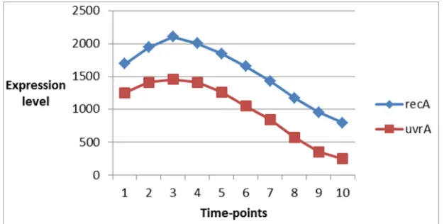
time-point or experimental conditions. Figure 1 shows the

expression patterns of two genes recA and uvrA in ecoli

dataset having the same trend, while figure 2 shows the

expression patterns of uvrA and uvrY having different trend.

Figure 3 shows a mixed regulation patterns. Expression trend measures are used to build the contingency table for two genes so as to calculate the adjusted rank index for the genes, which is used to determine whether they are co-expressed or not (details in section 4). The local similarity approach measures the expression trend of 2 the two genes at the same

time-point/condition. That is, the expression pattern of gene

X and gene Y at (X1, Y1), (X2, Y2), (X3, Y3)….. (Xn, Yn). The

global similarity check considers the expression pattern of

(X1, Y2), (X1, Y3), (X1, Y4)….. (X1, Yn),to further reinforce the

analysis and observation of expression trend of the two genes.

This is done to every sample of each gene against samples of the other gene. The global similarity check has little impact on the outcome of the similarity measure unlike the local similarity check.

Figure 1. Expression patterns of two genes recA and uvrA in ecoli dataset having the same expression trend.

Figure 2. Expression patterns of two genes recA and uvrA in ecoli dataset having the different expression trend.

(4)

3. Method

The approach used for the discovering of gene expression modules is to iteratively rank each gene against other genes to generate a rank matrix that will represent the level of expression trends each gene has with others. The statistical and computational model used to achieve this is called Fuzzified Adjusted Rand Index.

3.1. Fuzzified Adjusted Rand Index (FARI)

The traditional Adjusted Rand Index (ARI) is a data clustering metric that measures the similarity between two clustering results. It returns a single value indicating the level of agreement between two partitions. An ARI score of 1 indicates that the two clustering results are the same while 0 indicates that the two clustering results are not the same.

Computing ARI starts by building the Contingency Table

(similar to confusion matrix) for the two clusters. The contingency table is filled in by calculating the size of intersection of each group in the clusters against each other, which is formed by the number of items that are either in agreement or disagreement in the groups of the two clusters. However, it is impractical to get the measure of agreement of gene expression values because they are usually real values. In order to overcome this challenge, fuzzy concept of rule sets is incorporated in the process of building the contingency table.

ARI is given as:

, = (1)

where Index, MaxIndex and ExpectedIndex are calculated

from the contingency table built from the two clusters:

ARI = ∑ "$%#$%&' (∑ "$ )$&'∑ "% *%&'+/-#&.

//0(∑ "$)$_&'1∑ "%*%&'+ (∑ "$)$&'∑ "% *%&'+-#&. (2)

Where nij, ai, bj and n are values from the contingency

table:

-2

3., combination of m and k, for 1≤k≤m.

-2₃. = 0, for k<0, m<k.

3.2. Contingency Table Algorithm

The building of contingency table is very central to the use of adjusted rank index because all the values used in the calculation of the adjusted rand index are taken from the contingency table. A contingency table is a tabular form of relationship between variables filled in with integer numbers, which shows the level of agreement or disagreement among the categorical variables of the two clusters.

Given a set S of n elements, and two groupings or

partitions (clusters) of these points, i.e:

X = {x1, x2, ………., xr}

Y = {y1, y2, ………., ys}

The overlap/intersection between X and Y can be

summarized in a contingency table nij, each entry nijdenotes

the number of objects in common between Xi and Yj.

i.e, nij = |Xi∩Yj|

The overlap is a measure of proximity between a pair of genes across samples, showing the transcript levels of two co-expressed genes rising and falling together. Since gene expression data are real values; hence, it is difficult to calculate number of common objects in two gene sample profiles. Fuzzy rules concept is applied to eliminate this challenge, where levels of agreement of samples of a gene against other samples of the other gene are distributed into different bins and clusters. Different values (measures) representing class labels are attached to bins and clusters accordingly. Each value is then used to fill contingency table of two gene objects of different samples.

3.3. Building of Fuzzy Rules

The process to separate data into groups according to their respective class labels, which is the first step in fuzzy rule generation is perform by applying two conditions. The conditions are whether the two samples between a pair of genes are the same time-point or not. The first condition separates data into discrete interval (bins), while the second condition separates the data into clusters.

Given a pair of genes X and Y and the expression values

rescaled to interval [0, 1] by use of a linear transformation;

i. The first condition checks similar expression pattern of

two samples Xi and Yi.This is at the same experimental

condition or time point (i.e local similarity)

Let Xp and Yp be expression patterns of genes X and Y at

point i, we have two discrete values as class labels nij = 10

and nij= 0.

The membership function, which is the first step in fuzzy rule generation of these groups is constructed as follow:

Xp = exp (Xi – Xi-1

Yp = exp (Yi – Yi-1)

If (Xp>0 and Yp>0) OR (Xp<0 and Yp<0) Then:

nij= 10 > bin 1

Else,

nij = 0 > bin 2

where Xi-1 = 0.0 if i = 1.

ii.The second conditions checks similar expression pattern

of two samples Xi and Yj when i≠j. other similarity

across samples (i.e global similarity).

Let AD be the absolute difference (AD) of expression

values of genes X and Y at Xi and Yj when i≠j being the size

of their intersection, the values of the intersection are partitioned into six (6) different clusters as the class label

(5)

The membership function is constructed as follow;

AD = exp (|Xi – Yj|)

Table 1. The data point clusters defined for AD.

Data-points Clusters

0.00 – 0.049 Cluster 1

0.05 – 0.09 Cluster 2

0.10 – 0.19 Cluster 3

0.20 – 0.349 Cluster 4

0.35 – 0.49 Cluster 5

0.50 – 1.00 Cluster 6

nij = µAD: AD → [5, 4, 3, 2, 1, 0]

The values assigned to each partition shows the measure of agreement or disagreement between gene expression values, where the highest value indicates relatedness and lower value indicates disagreement. The ranges of partitions are assumed between 0 and 1 because the original gene expression data has been normalized between 0 and 1.

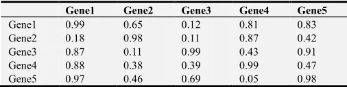
3.4. Generation of Rank Matrix

Application of FARI to construct gene expression modules from expression data is an iterative process, where the algorithm is applied to a pair of genes at a time. At every point of its application, a single value is returned signifying the level of closeness in expression trends of the two genes. This value is stored in a kind of an adjacency matrix before picking the next pair of genes to analyze, until all the gene objects are compared in pairs. The table below gives the description of the rank matrix.

Table 2. Description of a rank matrix. Each cell gives the rank value of similarity expression trend of a Gene in the row against another Gene in the column.

Gene1 Gene2 Gene3 Gene4 Gene5

Gene1 0.99 0.65 0.12 0.81 0.83

Gene2 0.18 0.98 0.11 0.87 0.42

Gene3 0.87 0.11 0.99 0.43 0.91

Gene4 0.88 0.38 0.39 0.99 0.47

Gene5 0.97 0.46 0.69 0.05 0.98

4. Result and Discussion

4.1. Co-expression Modules Construction

This work presents the power of a novel method called Fuzzified Adjusted Rank Index (FARI) to determine the magnitude of co-expression of a pair of genes among other several genes by checking similar expression pattern of two genes samples locally and globally. Local similarity determines the level of co-expression where a gene sample is at the same sample point or experimental condition with the other gene, while global similarity determines the level of co-expression a gene sample across samples or experimental conditions of the other gene. These metrics are used to determine the overall magnitude of co-expression of the pair

of genes. Input dataset used include a synthetic data, E. coli

SOS DNA repair data and Mtb microarray data (GSE11199) generated by Thuong et al. [15], which was updated in 2017. The experiment was to identify tuberculosis susceptibility genes from ex vivo Mtb-stimulated human macrophages. Gene expression levels of over 38,500 genes were measured in 12 subjects with 3 clinical phenotypes: latent, pulmonary, and meningeal TB (n = 4 per group), which contain probe

sets for 47,000 transcripts. A web server called g: Profiler (a

web server for functional interpretation of gene lists) was used to convert the probe IDs to their corresponding gene names and functional annotations after the co-expressed modules have been created. There are two categories of exceptional probe IDs, the first category is a set of few probe IDs that got converted to more than one gene names. This set of genes made the number of genes in some modules to be increased and they are treated the same as they were discovered to have the same functional annotation attached to them. The second category is the set of probe IDs, which their gene names are not available in the annotation database

and are indicated as N/A. These ones are filtered out of their

corresponding co-expression modules making the number of genes in some modules to be reduced.

Due to the size of the dataset and the number of genes

generated from this experiment, corroborated by Luo et al. [1]

that the process of identifying cellular network in an automatic and objective fashion from genome-wide expression data remain challenging, we investigated the co-expression of the genes in scales and ranges such as the first 100 genes or genes 500 – 850. We later analyzed the modules generated from different investigations to identify the hub genes and analyze the functional activities of the hub genes using an annotation databases. A gene module is a cluster of densely interconnected genes in terms of co-expression [2]. FARI analyses the expression patterns of the genes under investigation and produces a rank matrix showing different values that depict the magnitude of co-expression of each gene with all other genes.

The co-expression modules are constructed from each gene under investigation. That is, for each gene, we extract the genes that have the same expression pattern with it using the rank matrix produced by FARI. So, four or eight co-expressed genes are extracted for each gene as a target to form a gene co-expressed module. This procedure is based on three factors; firstly, owning to the submissions that modular co-expression network structure and topology (number, size, content and connection) are subjective depending on the threshold chosen, secondly that co-expressed genes do interact together [1, 5], and thirdly that each gene is estimated on average to interact with four (in bacterial and prokaryotes) to eight (in Eukaryotes) other genes [2].

4.2. Analysis of the Rank Matrix with Synthetic Data and E. coli SOS DNA Repair Data

(6)

computational model developed to do this analysis, which produces rank matrix of values depicting the levels of co-expression of each gene with other genes. Two dataset are used to examine and validate the efficiency of our model, the first is five (5) synthetic noiseless gene expression dataset containing 30 genes with 50 time-points, containing 250

samples altogether [11]. The second is E. coli SOS DNA

repair dataset containing 8 genes with 50 samples [11-13]. After proper inspection of the rank matrix generated from the two datasets, we discovered that the diagonal values are mostly the highest values across each row. These are the rank values gotten when expression pattern of a gene is analyzed

against itself because the process is automated. It is instructive to know that the traditional Adjusted Rank Index from which our model is developed produces values between 1 and 0 when used to compare clustering results, and gives 1 when the clustering results are closely related while it gives 0 when they are not related at all. Going by this fact, we normalized the initial rank matrix produced between 0 and 1 in order to represent the true picture of the expression pattern.

Table 3 shows the rank matrix generated for ecoli while

the synthetic gene expression dataset is given in the supplementary file.

Table 3. Rank Matrix of Ecoli SOS DNA repair data.

uvrD lexA umuDC recA uvrA uvrY ruvA polB

uvrD 1.0000 0.2644 0.0000 0.2155 0.1147 0.5949 0.3439 0.3197

lexA 0.6280 1.0000 0.0000 0.1254 0.3040 0.7783 0.5437 0.4007

umuDC 0.1554 0.0042 1.0000 0.1708 0.0914 0.0000 0.3515 0.9280

recA 0.6941 0.5908 0.0000 1.0000 0.6423 0.5698 0.5650 0.8359

uvrA 0.2825 0.1390 0.0325 0.0631 0.9451 0.5480 0.0000 1.0000

uvrY 0.4123 0.1935 0.0000 0.1930 0.0549 1.0000 0.4560 0.3096

ruvA 0.7370 0.4303 0.3723 0.4403 0.2915 0.5993 1.0000 0.0000

polB 0.2608 0.2490 0.3275 0.5930 0.3704 0.2254 0.0000 1.0000

4.3. Co-Expression Modules and Networks from the Ecoli SOS DNA Repair Data

Identification of co-expression modules in particular gene expression dataset involves the process of grouping the genes with the same expression pattern into different clusters. Our method found the number of clusters being equivalent to the number of genes under investigation because the expression patterns were analyzed per each gene. Moreover, each module contains not greater than five genes because each gene is estimated on average to interact with four (in

bacterial and prokaryotes) to eight (in Eukaryotes) other

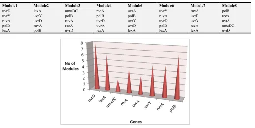
genes [2]. Table 4 shows different modules from Ecoli SOS

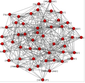
DNA repair data while Figure 4 shows the frequency of each

gene in modules. uvrY, uvrD and polB are suspected to be the

hub genes, which is established with the co-expression network (Figure 5) constructed from the module. We query this discovery by searching the E. coli SOS DNA repair

network genes on KEGG database

(https://www.genome.jp/kegg/pathway.html ) and discovered that these genes engage in more pathway networks than all other genes as shown in Table 5.

Table 4. Co-expression Modules of Ecoli SOS DNA Repair Data.

Module1 Module2 Module3 Module4 Module5 Module6 Module7 Module8

uvrD lexA umuDC recA uvrA uvrY ruvA polB

uvrY uvrY polB polB polB ruvA uvrD recA

ruvA uvrD ruvA uvrD uvrY uvrD uvrY uvrA

polB ruvA recA uvrA uvrD polB recA umuDC

lexA polB uvrD lexA lexA lexA lexA uvrD

(7)

Figure 5. Co-expression network of Ecoli SOS DNA Repair Data.

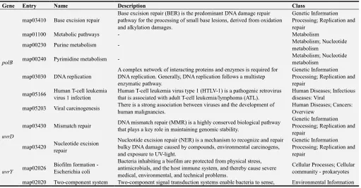
Table 5. KEGG Pathways of E. coli SOS DNA Repair Network.

Gene Entry Name Description Class

polB

map03410 Base excision repair

Base excision repair (BER) is the predominant DNA damage repair pathway for the processing of small base lesions, derived from oxidation and alkylation damages.

Genetic Information Processing; Replication and repair

map01100 Metabolic pathways - Metabolism

map00230 Purine metabolism - Metabolism; Nucleotide

metabolism

map00240 Pyrimidine metabolism - Metabolism; Nucleotide

metabolism

map03030 DNA replication

A complex network of interacting proteins and enzymes is required for DNA replication. Generally, DNA replication follows a multistep enzymatic pathway.

map05166 Human T-cell leukemia virus 1 infection

Human T-cell leukemia virus type 1 (HTLV-1) is a pathogenic retrovirus that is associated with adult T-cell leukemia/lymphoma (ATL).

Human Diseases; Infectious diseases: Viral

map05203 Viral carcinogenesis There is a strong association between viruses and the development of human malignancies.

Human Diseases; Cancers: Overview

uvrD

map03430 Mismatch repair DNA mismatch repair (MMR) is a highly conserved biological pathway that plays a key role in maintaining genomic stability.

map03420 Nucleotide excision repair

Nucleotide excision repair (NER) is a mechanism to recognize and repair bulky DNA damage caused by compounds, environmental carcinogens, and exposure to UV-light.

uvrY map02026

Biofilm formation - Escherichia coli

Bacteria inhabiting a biofilm are protected from physical stress, antimicrobials, and the host immune system, and thereby cause severe medical, environmental, and technical problems.

Cellular Processes; Cellular community - prokaryotes

(8)

Gene Entry Name Description Class respond, and adapt to changes in their environment or in their intracellular state.

Processing; Signal transduction

map02025

Biofilm formation - Pseudomonas aeruginosa

Surface colonization and subsequent biofilm formation and development provide numerous advantages to microorganisms.

map05111 Biofilm formation - Vibrio cholerae

Surface colonization and subsequent biofilm formation and development provide numerous advantages to microorganisms.

recA map03440 Homologous

recombination

Homologous recombination (HR) is essential for the accurate repair of DNA double-strand breaks (DSBs), potentially lethal lesions. It is investigated that RecA/Rad51 family proteins play a central role.

uvrA map03420 Nucleotide excision repair

Nucleotide excision repair (NER) is a mechanism to recognize and repair bulky DNA damage caused by compounds, environmental carcinogens, and exposure to UV-light.

4.4. Co-Expression Modules and Networks from the Mtb-Stimulated Human Macrophages Data

Due to the size of the dataset and the number of the genes generated from the experiment, we investigated different co-expression of the experiment in ranges of gene sets; where each set represent the input data of each investigation. We decided to break the dataset into subsets based on regions because Gene-to-Gene analysis has shown that the biochemical activities within a region in DNA sequence are functions of contributions of individual gene within the neighbourhood [19]. That is, the genomic location has some impact on gene expression which generally has influence on the gene function within a framework of expression defined by that neighbourhood. The theoretical study, [18] listed gene neighbourhood as one of the factors that affect gene expression but was quick to assume that the existence of gene expression neighbourhoods is not necessary for the correct and coordinated expression of genes that have the same expression profiles. The gene sets are described in Tables 6 and 7 below, where each is used to generate different co-expression modules.

Table 6. Details of the Data Inputs in Scales.

S/N Gene Scales in the Dataset No of Gene

1 1 – 50 50

2 1 – 100 100

3 1 – 200 200

4 1 – 350 350

5 1 - 500 500

Table 7. Details of the Data Inputs in Ranges.

S/N Gene Scales in the Dataset No of Gene

1 1 – 350 350

2 101 – 450 350

3 201 – 550 350

4 301 – 650 350

5 401 – 750 350

6 501 – 850 350

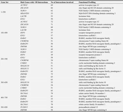
The breaking down of the original dataset gives us 11 input datasets, which is just a fractional part of the original dataset. Table 6 gives the dataset in scales, which describes the scope and magnitude of gene coverage of the original dataset (i.e the first 50, 100, 200, 350 and 500 genes). Table 7 describes the input dataset in ranges from the original dataset, which is in form of interval data points at the size of 350 genes per interval (i.e from 1-350, 101-450, 201-550, 301-650, 401-750 and 501-850). This procedure is employed in order to appropriately capture the hub genes in the dataset from the co-expression modules, by comparing the co-expression modules at different scales and ranges instead of using the whole dataset at once that could lead to under-representation of the underline expression pattern due to the size of the dataset and the potential noise in the data. Only the first 500 genes from the original dataset were investigated using the scaled datasets while the first 850 genes were investigated using the datasets by ranges.

4.5. Analysis of Hub Genes

(9)

Figure 6. Frequency of each gene participating in co-expression modules of 1-50 Genes in the Dataset.

Figure 7. Co-expression network of 1-50 Genes in the Dataset.

The results from the scaled datasets shows that that the hub genes discovered when small dataset is used are also parts of the hub genes when large dataset is used, though not as highly connected as others in the large dataset. They include PTPN21, CNOT7, FAM122C, MSANTD3, LEAP2, GIMAP1, GAPT, AK9, UBA7, MIR4435-2HG, RBBP6, PXK, CFAP53, SCARB1, CCDC65, C4ORF33, FAM71A, MIR5193.

4.6. Functional Analysis of Identified Hub Genes

The functional activities that the most common (real) hub genes engage in were identified through an annotation

database called g: profiler. We decided to analyze the hub

(10)

Table 8. Functional activities of most common hub genes.

Gene Functional Activities

KNL1 kinetochore scaffold 1

CNBD2 cyclic nucleotide binding domain containing 2

ABRA actin binding Rho activating protein

SLC2A13 solute carrier family 2 member 13

USP28 ubiquitin specific peptidase 28

ARL11 ADP ribosylation factor like GTPase 11

SLC4A1 solute carrier family 4 member 1

RXFP1 relaxin family peptide receptor 1

CNBD2 cyclic nucleotide binding domain containing 2

Gene Functional Activities

ARPP21 cAMP regulated phosphoprotein 21

CARD16 caspase recruitment domain family member 16

ZMYM6 zinc finger MYM-type containing 6

TAF1L TATA-box binding protein associated factor 1 like

RECQL4 RecQ like helicase 4

DEFB105B defensin beta 105B

HAS3 hyaluronan synthase 3

CBLL2 Cbl proto-oncogene like 2

DEFB105A defensin beta 105A

Table 9. Functional activities of hub genes with highest interactions in each dataset.

Gene Set Hub Genes with >50 Interactions No of Interactions involved Functional Profiling

1-350

ACVR1C 69 activin A receptor type 1C

ZSCAN20 66 zinc finger and SCAN domain containing 20

NLRC4 62 NLR family CARD domain containing 4

MSANTD3 53 Myb/SANT DNA binding domain containing 3

LACTB 53 lactamase beta

KNL1 50 kinetochore scaffold 1

101-450

ACVR1C 72 activin A receptor type 1C

ZSCAN20 71 zinc finger and SCAN domain containing 20

LACTB 59 lactamase beta

RTP3 57 receptor transporter protein 3

RAB42 56 RAB42, member RAS oncogene family

C9ORF66 51 chromosome 9 open reading frame 66

RAB42P1 56 RAB42, member RAS oncogene family, pseudogene 1

201-550

ZMYM6 81 zinc finger MYM-type containing 6

RTP3 59 receptor transporter protein 3

CNBD2 51 cyclic nucleotide binding domain containing 2

SIGLEC10 51 sialic acid binding Ig like lectin 10

301-650

CNBD2 51 cyclic nucleotide binding domain containing 2

401-750

SLC36A1 78 solute carrier family 36 member 1

501-850

SLC36A1 70 solute carrier family 36 member 1

PCDH15 64 protocadherin related 15

5. Conclusion

Although, co-expression module techniques generally depend on proximity measures based on global similarity to draw the relationship between genes, but it is observed that

(11)

co-expression modules in Mtb data, which is used to

construct co-expression networks from which

highly-connected genes are characterized by their functions. FARI gives us an insight into the relationship between genes, which eventually gives us the opportunity to pick the most

plausible genes as the best combination of

affecting/regulatory genes in constructing gene regulatory network unlike creating hypothetical connections by using conditional combinations of gene as input in the study or using constraint to prune the network in these studies [10-12].

Meanwhile, further analysis could include the enrichment analysis of the gene modules using Kyoto Encyclopedia of Genes and Genome (KEGG) and Gene Ontology (GO) databases. Also parallelism could be incorporated into FARI so that the comparison of gene pairs would be done simultaneously according to the computing power of the machine instead of iteratively.

References

[1] Luo F., Yang Y., Zhong J., Gao H., Khan L., Thompson D. K. and Zhou J.(2007). Constructing gene co-expression networks and predicting functions of unknown genes by random matrix theory. BMC Bioinformatics, 8: 299 doi: 10.1186/1471-2105-8-299.

[2] Li J., Zhou D., Qiu W., Shi Y., Yang J., Chen S., Wang Q. and Pan H.(2018). Application of Weighted Gene Co-expression Network Analysis for Data from Paired Design. Scientific Reports | (2018) 8: 622 | DOI: 10.1038/s41598-017-18705-z. [3] Jiang J., Sun X., Wu W., Li L., Wu H., Zhang L., Yu G. and

Li Y. (2016). Construction and application of a co-expression network in Mycobacterium tuberculosis. Scientific Reports | 6: 28422 | DOI: 10.1038/srep28422.

[4] Ruan J., Dean A. K., and Zhang W.(2010). A general co-expression network-based approach to gene expression analysis: comparison and applications. BMC Systems Biology 2010, 4: 8.

[5] Roy S., Bhattacharyya D. K., and Kalita J. K. (2014). Reconstruction of gene co-expression network from microarray data using local expression patterns. BMC Bioinformatics 2014, 15 (Suppl 7): S10.

[6] Ballouz S., Verleyen W. and Gillis J. (2015). Guidance for RNA-seq co-expression network construction and analysis: safety in numbers. Bioinformatics, 31 (13), 2015, 2123–2130 doi: 10.1093/bioinformatics/btv118.

[7] Gibson S. M., Ficklin S. P., Isaacson S., Luo F., Feltus F. A. and Smith M. C. (2013). Massive-Scale Gene Co-Expression Network Construction and Robustness Testing Using Random Matrix Theory. PLoS ONE 8 (2): e55871. doi: 10.1371/journal.pone 0055871.

[8] Song L., Langfelder P. and Horvath S. (2012). Comparison of co-expression measures: mutual information, correlation, and model based indices. BMC Bioinformatics 2012, 13: 328.

[9] Villa-Vialaneix N., Liaubet L., Laurent T., Chere P., Gamot A. and SanCristobal m. (2013). The Structure of a Gene Co-Expression Network Reveals Biological Functions Underlying eQTLs. PLoS ONE 8 (4): e60045. doi: 10.1371/journal.pone.0060045.

[10] Grimaldi, M., Visintainer, R. and Jurman, G. (2011). RegnANN: Reverse Engineering Gene Networks Using Artificial Neural Networks. PLoS ONE, Vol. 6, Issue 12, e28646.

[11] Mandal S., Khan A., Saha G., and Pal R. K. (2016) Large-Scale Recurrent Neural Network Based Modelling of Gene Regulatory Network Using Cuckoo Search-Flower Pollination Algorithm. Advances in Bioinformatics Volume 2016, Article ID 5283937, 9 pages.

[12] Raza K. and Alam M. (2016) Recurrent Neural Network Based Hybrid Model of Gene Regulatory Network. Computational Biology and Chemistry, 64: 322-334.

[13] Noman N., Palafox L., and Iba H., (2013) “Reconstruction of gene regulatory networks from gene expression data using decoupled recurrent neural network model,” in Natural Computing and Beyond: Winter School Hakodate 2011, Hakodate, Japan, March 2011 and 6th International Workshop on Natural Computing, Tokyo, Japan, March 2012, Proceedings, vol. 6 of Proceedings in Information and Communications Technology, pp. 93–103, Springer, Berlin, Germany, 2013.

[14] Reimand, J., Arak, T., Adler, P., Kolberg, L., Reisberg, S., Peterson, H., Vilo, J. g: Profiler - a web server for functional interpretation of gene lists (2016 update) Nucleic Acids Research 2016; doi: 10.1093/nar/gkw199.

[15] Thuong NTT, Dunstan SJ, Chau TTH, Thorsson V, Simmons CP, et al. (2008) Identification of Tuberculosis Susceptibility Genes with Human Macrophage Gene Expression Profiles. PLoS Pathog 4 (12): e1000229. doi: 10.1371/journal.ppat.1000229.

[16] Farahbod F. and Eftekhari M. (2013) A New Clustering-Based Approach for Modeling Fuzzy Rule-Based Classification Systems. IJST, Transactions of Electrical Engineering, Vol. 37, No. E1, pp 67-77.

[17] Priyono A., Ridwan M., Alias A. J., Rahmat R. A. O. K., Hassan A. and Ali M. A. M. (2005). Generation of Fuzzy Rules with Subtractive Clustering. Jurnal Teknologi, 43 (D) Dis. 2005: 143–153.

[18] Jones R (2010) There Goes the (Gene Expression) Neighbourhood Theory. PLoS Biol 8 (11): e1001002. doi: 10.1371/journal.pbio.1001002.

[19] Oliver B., Parisi M. and Clark D. (2002). Gene expression neighborhoods. Journal of Biology 2002, Volume 1, Issue 1, Article 4. http://jbiol.com/content/1/1/4.