SUB-DOMAIN MOM FORMULATION
FOR CIRCULAR AND NON-CIRCULAR
LOOP ANTENNA ARRAYS
TOMÁŠ PÁLENÍK
Department of Measurement, Slovak University of Technology in Bratislava, Ilkovičova 3 Bratislava 812 19, Slovakia
MIKULÁŠ BITTERA
Department of Measurement, Slovak University of Technology in Bratislava, Ilkovičova 3 Bratislava 812 19, Slovakia
VIKTOR SMIEŠKO
Department of Measurement, Slovak University of Technology in Bratislava, Ilkovičova 3 Bratislava 812 19, Slovakia
Abstract:
The method of moments (MoM) analysis of thin-wire loop antenna arrays with multiple elements is presented in this paper. The proposed formulation provides simple algorithmic implementation that can be applied to circular loop arrays as well as more generally shaped arrays using the Pocklington’s integral equation with simplified kernel for arbitrary shaped wires in combination with a superquadric curve representation. This analysis leads to knowledge of the current distribution, input impedance and other electromagnetic properties of both uniform and non-uniform loop arrays. Numerical results are included to exhibit good agreement with various relevant references and simulation software. The data for large square and rectangular loop arrays are presented for the first time in literature.
Keywords: Current distribution; integral equation; method of moments; loop antenna arrays.
1. Introduction
Circular loop antennas present a basic antenna type that can be arranged into antennas arrays with improved properties. Such arrays have been studied by several authors [Ito et al. (1971)], [Shoamanesh and Shafai (1978, 1979)], [Huang et al. (2003)] or [Krishnan et al. (2005)] using the solution technique based on the integral equation by means of Fourier series expansion. In contrary to this technique, there is an alternative approach [Papakanellos et al. (2010)] still based on the integral equation method however in conjunction with the sub-domain method of moments (MoM). This approach uses integral equations that are discretized via step-pulse (pulse triplet) basis functions with point matching technique. It is shown that such approach is simpler in implementation than Fourier series method and it supports straightforward modification of wire antenna excitation models which may feed any one of the array of elements.
processing units [De Donno et al (2010)] to achieve higher computing performance for large antenna arrays. In this paper, the piecewise sinusoidal basis and testing functions (Galerkin’s method) are chosen for better results accuracy at the cost of greater computation time.
2. Pocklington’s Integral Equation
Note that thin-wire assumption holds throughout the paper supposed that the wire radius of loop is much smaller than the wavelength at the frequency of operation and the length of wire. Under this condition, the surface current density on the wire can be assumed as axial filamentary current. In this case, the general form of Pocklington’s integral equation that relates the unknown total axial current I(s’) to the axial component of the known impressed electric field from the antenna feeding source Ei(s) on the surface is given by
− • + ∂ ∂ ∂ − = L i ds R jkR e s s k s s s I j sE ' '
' ) ' ( 4 1 ) ( 2 2 ωε π (1) where L is circumference of the curved-wire structure, k=2π/λ is the wave number, ω is the angular frequency, ε is the permittivity of the surrounding medium, s is the unit tangential vector along the wire axis and s' is the unit tangential vector in direction of the co-ordinates s and s’, respectively. The distance R from (1) between the source and observation point is given by
'
r r R= −
(2) where the vector equation for the wire axis as places of the observation points can be expressed using unit
vectors i,j,k as
k z j y i x
r= + + (3)
and the equation for the parallel curve that represents the current filament on the wire surface can be expressed as
n r r r'= + 0
(4) where r0 is the wire radius and nis the normal unit vector along the wire axis. This curve configuration
overcomes the problem with singular integral when source and observation points coincide. The kernel simplification [Figureoa et al. (2004)] that eliminates the second derivative from (1) for arbitrary shaped wire structures yields
− • • − + + • − − − = L jkR i ds R e s R s R R k jkR s s jkR R k R s I j s E ' ) ' )( )( 3 3 ( ' ) 1 ( ) ' ( 4 1 ) ( 5 2 2 2 2 2 ωε π . (5) It invokes only elementary mathematical operations.2.1. Superquadric representation
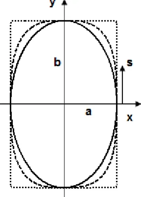
The superquadric curve satisfies the following equation
1 = + v v b y a x (6) where a and b are the semiaxes in the x and y directions respectively, and v is the squareness parameter. A
values of v=2 and b/a=1 correspond to a circle.
Fig. 1 illustrates the superquadric curve for v = 2, 3, 50 and an aspect ratio b/a=2. Note that loop squareness is increased with v. The Eq. (6) allows to model circle, ellipse, square and rectangle loops flexibly. Hence for circular as well as non-circular loops, the idea of superquadric curve can be applied to represent vector equations for wire axis r and parallel curve r’ defined by (3) and (4), respectively, using an alternative representation of the superquadric curve that can be given as in [Jensen and Rahmat-Samii (1994)]
where
v v v
1
) cos sin
(
1 )
(
Φ + Φ = Φ Ψ
(8) and the angle parameter Φ is in the range 0 ≤Φ≤ 2π. The unit tangential vector is obtained as
Φ Φ
+
Φ Φ
− Φ = +
= −
−
j b
i a
j s i s s
v v
y x
) sgn(cos cos
) sgn(sin sin
) (
1
1 1
γ
(9) where
2 2 2 2 2 2
cos sin
)
(Φ = a Φ v− +b Φ v− γ
. (10) The differential arc length ds along the wire axis can be expressed in terms of the differential dΦ letting
Φ Φ Δ
= d
ds ( )
(11) where
) ( ) ( )
(Φ = Φ Ψ 1 Φ
Δ γ v+
. (12) On solving the simplified Pocklington’s integral equation (5) with superquadric wire representation, the MoM [Balanis (2008)] can be applied to convert it into algebra matrix equations. To provide the computation with loop antenna arrays, the formulation has to be further extended with mutual interactions between elements as is proposed in the following section.
Fig. 1. Superquadric curve with aspect ratio b/a=2 for v=2 (solid line), v=3 (dashed line) and v=50 (dotted line)
3. Proposed Method of Moments Solution of Thin-Wire Array of Loops
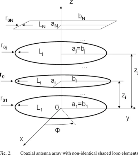
Consider N superquadric loop antennas with arbitrary semiaxes a1, a2,…ai,…aj,…aN and b1, b2,…bi,…bj,…bN with arbitrary squareness parameters v1, v2,…vi,…vj,…vN which are constructed from a perfectly conducting thin wires of radius r01, r02, … r0i, … r0j, …r0N arranged parallel to each other with the centers on the z axis. This consideration supports arrays computation with non-identical loop elements, as is illustrated in Fig. 2, where the values z1, z2,…zi,…zj,…zN denote the element spacing from the reference.
To apply the sub-domain MoM, each loop is subdivided into X segments and the current on a wire is approximated by a linear combination of basis functions fn(Φ) in form
( )
( )1
, Φ
=
Φ
=
n X
n n i
i I f
I
where Ii,n is the nth unknown basis function weighting coefficient associated with ith loop.
Fig. 2. Coaxial antenna array with non-identical shaped loop elements
The piecewise sinusoidal basis functions spanning two segments used in the paper have the form
Φ ≤ Φ ≤ Φ Φ
− Φ
Φ − Φ
Φ ≤ Φ ≤ Φ Φ
− Φ
Φ − Φ
=
Φ +
+ +
− −
−
elsewhere if if
f n n
n n
n
n n
n n
n
n
, 0
, ) sin(
) sin(
, ) sin(
) sin(
)
( 1
1 1
1 1
1
(14) and the same holds for the sinusoidal testing functions with subscripts m. The resulting matrix equation describing the array of loops with account to mutual coupling effects can be expressed in matrix form symbolically as
[ ] [ ][ ]
V = Z I (15)where generalized voltage column matrix [V] is given as
[
]
TX N N N X
X V V V V V V
V V V
V] 1,1, 1,2,... 1, , 2,1, 2,2,... 2, ,...., ,1, ,2,... , [ =
(16)
where the first subscript represents the loop number and the second one the number of segment. Generalized current column matrix [I] has the subsequent form
[
]
TX N N N X
X I I I I I I
I I I
I] 1,1, 1,2,...1, , 2,1, 2,2,...2, ,...., ,1, ,2,... , [ =
(17) and the generalized mutual impedance matrix has the form
[ ]
=
NN N
N
N N
Z Z
Z
Z Z
Z
Z Z
Z
Z
2 1
2 22
21
1 12
11
X m for d E f
Vim m i ii
m m ...., 3 , 2 , 1 , ) ( ) ( ) ( 1 1 , =
Φ Φ Φ ΔΦ Φ = + − ΦΦ (19)
and elements of submatrix Zij from (18) are given by
[ ]
X 1,2,..., n and X 1,2,..., m , ' ) ' ( ) ( ) ' ( ) ( 4 1 1 1 1 1 = = Φ Φ Φ Δ Φ Δ Φ Φ − =
+ − + − Φ Φ Φ Φ for d d T f f jZmn ij m n ij
m m n n ωε π (20) for each combination of i=1,2,…,N and j=1,2,…,N. The term Tij is derived from (5) and has the form
5 2 2 2 2 2 ) 3 3 )( ' ( ) ( ' ) 1 ( ij jkR ij ij j ij i ij j i ij ij ij ij R e R k jkR s R s R s s jkR R k R T ij − − + • • + • − − = (21)
where Rij represents the distance from the observation point on the loop Li to the source point on the loop Lj. In
the case that holds i=j the convention for places of observation and source points from Section 1 holds, otherwise the source point and observation point can be due to thin-wire assumption chosen on the wire axis on both loops. To model the field Ei in (19), one can choose from a set of standard used feed models [Balanis (2008)], e.g. delta-gap generator or magnetic frill. Once the excitation has been properly described, the MoM analysis can be carried out and approximate current distribution in discrete form (17) can be proceed with an inversion of Z matrix. Then one can straightforward determines the input impedance [Páleník et al. (2010)] or the input admittance, radiation pattern [Hajach and Harťanský (2003)], gain and other electromagnetic parameters of investigated arrays from this distribution.
4. Numerical Results
To ascertain the accuracy of the proposed formulation, the computed results based on aforementioned sections are compared with results reported in [Shoamanesh and Shafai (1979)] and [Papakanellos et al. (2010)], in which the non-uniform Yagi arrays are investigated. The arrays consist of a reflector kb1=1.05, an exciter
kb2=1.1, and the various number of directors (see first column in Table 1) with kbi=0.9 where bi denotes radius
of circular loops for which the semiaxes are equal in length ai=bi. The wire radius is set to Ω=2ln(2πb2/r0)=11
for each array element. The distance between the reflector and the exciter is taken to be Δz=0.1λ and the director spacing is equally set to Δz=0.2λ. Exciting element is excited at Φ=0 by a unit delta-gap voltage source. The computed input admittances are shown in Table 1 where each array element is modeled with 100 segments. One can see that the computed admittances are in good agreement with referenced values.
Number of directors
Input admittance (mS)
Computed values
Reference data from [Shoamanesh and Shafai
(1979)]
Reference data
from [Papakanellos et al. (2010)]
2 1.628-j5.250 1.60-j5.18 1.678-j5.208
4 1.561-j5.451 1.56-j5.38 1.615-j5.421
6 1.548-j5.650 1.54-j5.58 1.611-j5.629
8 1.620-j5.852 1.61-j5.78 1.698-j5.836
9 2.130-j5.170 2.13-j5.10 2.162-j5.112
10 1.801-j6.016 1.80-j5.95 1.903-j5.993
Table 1. Input admittances for the Yagi arrays of non-uniform circular loops
Further results of uniform arrays of circular loops can be compared with data from [Papakanellos et al. (2010)]. The array consist of identical circular loops with bi = 0.15λ and r0i=0.01λ and with element spacing Δz=0.2λ. A
magnetic frill generator is implemented for a 50Ω air-filled feeding coaxial cable (outer radius a0=2.3r0) and it is
Number of elements
Input admittance (mS) Computed
values
Reference data
from [Papakanellos et al. (2010)] 5 3.510+j8.314 3.660+j8.642 7 4.408+j11.937 4.475+j12.314 9 3.206+j8.560 3.359+j8.872 11 4.814+j12.023 4.839+j12.405 13 2.995+j8.668 3.153+j8.959 15 5.149+j12.010 5.124+j12.498 17 2.860+j8.742 3.023+j9.009 19 5.452+j12.136 5.369+j12.562 21 2.782+j8.819 2.949+j9.064
Table 2. Input admittances for the uniform arrays of circular loops
Data for uniform arrays with square elements are shown in Table 3. The antenna arrays consist of square loops (ratio b/a=1 and v=50) with the identical perimeter and wire radius as in the previous case. Element spacing and magnetic frill generator parameters also hold with any changes. Since the data for such configurations are presented for the first time in literature, the computed values are compared with numerical data obtained from electromagnetic simulation software FEKO. In both cases, each loop element consists of 60 segments and results showing close agreement.
Number of elements
Input admittance (mS) Computed
values
FEKO values
5 2.369+j6.229 2.376+j6.244
7 1.570+j6.631 1.576+j6.625
9 2.428+j6.496 2.425+j6.515
11 1.599+j6.479 1.609+j6.473
13 2.355+j6.787 2.340+j6.802
15 1.659+j6.328 1.675+j6.323
17 2.113+j6.962 2.094+j6.961
19 1.790+j6.183 1.814+j6.183
21 1.853+j6.950 1.839+j6.938
Table 3. Input admittances for the uniform arrays of square loops
Finally, consider the case of rectangular loop array where for each element holds ratio b/a=2 and v=50 and the perimeter of rectangular remains as in previous case.
Number of elements
Input admittance (mS) Computed
values
FEKO values
5 2.807+j5.642 2.849+j5.657
7 4.432+j9.297 4.320+j9.269
9 2.391+j6.135 2.437+j6.118
11 5.699+j9.143 5.457+j9.196
13 2.164+j6.534 2.221+j6.485
15 6.863+j8.233 6.560+j8.524
17 2.065+j6.907 2.097+j6.826
19 7.259+j6.638 7.154+j7.205
21 2.066+j7.282 2.083+j7.167
Table 4. Input admittances for the uniform arrays of rectangular loops
5. Conclusion
In this paper, the Pocklington’s integral equation with simplified kernel for arbitrary shaped wires is used in combination with the superquadric curve. This leads to simple and efficient numerical procedure to investigate the circular, elliptical, square and rectangular loops in application with method of moments. This approach is further extended to compute large coaxial antenna arrays considering the mutual effects between loop elements. It can be concluded that the implemented procedure is sufficient to represent the current distributions and derived electromagnetic parameters for both circular and non-circular arrays although the computation is based on elementary mathematical operations. Presented numerical results for uniform and non-uniform circular loop antenna arrays are generally in close agreement with the various references. First time presented data for square and rectangular loop antenna arrays corresponds to that obtained from simulation software based on non-parametric geometry representation of wire antennas.
Acknowledgements
This research was financially supported by the project VEGA VG 1/0551/09. References
[1] Balanis, C. A. (2008). Modern Antenna Handbook. John Wiley & Sons, Inc.
[2] De Donno, D., et al. (2010). Parallel efficient method of moments exploiting graphics processing units. Microwave and Optical Technology Letters, 52(11), pp. 2568–2572.
[3] EM Software & Systems, FEKOSuite v5.5. Available at http://www.feko.info.
[4] Figureoa, V. B., Pedroza, J.S., Bonilla, J.L.L. (2004). Simplification of Pocklington’s Equation Kernel for Arbitrary Shaped Thin Wires. Revista Cubana De Fisica, 21(1), pp. 21-28.
[5] Hajach, P., Harťanský, R. (2003) Resistively Loaded Dipole Characteristics. Radioeng., 12(1), pp. 19-22.
[6] Huang, Y., Nehorai, A., Friedman, G. (2003). Mutual coupling of two collocated orthogonally oriented circular thin-wire loops. IEEE Transactions on Antennas and Propagation, 51(6), pp. 1306–1314.
[7] Ito, S., Inagi, N., Sekiguchi, R. (1971). An investigation of the array of circular-loop antennas. IEEE Transactions on Antennas and Propagation, 19(4), pp. 469-476.
[8] Jensen, M.A., Rahmat-Samii, Y. (1994). Characterization of electromagnetically coupled superquadric loop antennas for mobile communications applications. IEE Proc. Microw. Antennas Propag, 141(2), pp. 85-93.
[9] Krishnan, S., Li, L.W, Leong, M.S. (2005). Entire domain MoM analysis of an array of arbitrarily oriented circular loop antennas: A general formulation. IEEE Transactions on Antennas and Propagation, 53(9), pp. 2961–2968.
[10] Shoamanesh, A., Shafai, L. (1978). Properties of coaxial loop arrays. IEEE Transactions on Antennas and Propagation, 1978, 28(4), pp. 547-550.
[11] Shoamanesh, A., Shafai, L. (1979). Design Data for Coaxial Yagi Array of Circular Loops. IEEE Transactions on Antennas and Propagation, 27(5), pp. 711-713.
[12] Papakanellos, P.J., Tsitsas, N.L., Anastassiu, H.T. (2010). Efficient Modeling of Radiation and Scattering for a Large Array of Loops. IEEE Transactions on Antennas and Propagation, 58(3), pp. 999 - 1002.