University of Pennsylvania
ScholarlyCommons
Publicly Accessible Penn Dissertations
1-1-2015
Extensions and Applications of Ensemble-of-trees
Methods in Machine Learning
Justin Bleich
University of Pennsylvania, [email protected]
Follow this and additional works at:http://repository.upenn.edu/edissertations Part of theStatistics and Probability Commons
This paper is posted at ScholarlyCommons.http://repository.upenn.edu/edissertations/1016
For more information, please [email protected]. Recommended Citation
Bleich, Justin, "Extensions and Applications of Ensemble-of-trees Methods in Machine Learning" (2015).Publicly Accessible Penn
Dissertations. 1016.
Extensions and Applications of Ensemble-of-trees Methods in Machine
Learning
Abstract
Ensemble-of-trees algorithms have emerged to the forefront of machine learning due to their ability to generate high forecasting accuracy for a wide array of regression and classification problems. Classic ensemble methodologies such as random forests (RF) and stochastic gradient boosting (SGB) rely on algorithmic procedures to generate fits to data. In contrast, more recent ensemble techniques such as Bayesian Additive Regression Trees (BART) and Dynamic Trees (DT) focus on an underlying Bayesian probability model to generate the fits.
These new probability model-based approaches show much promise versus their algorithmic counterparts, but also offer substantial room for improvement. The first part of this thesis focuses on methodological advances for ensemble-of-trees techniques with an emphasis on the more recent Bayesian approaches. In particular, we focus on extensions of BART in four distinct ways. First, we develop a more robust implementation of BART for both research and application. We then develop a principled approach to variable selection for BART as well as the ability to naturally incorporate prior information on important covariates into the algorithm. Next, we propose a method for handling missing data that relies on the recursive structure of decision trees and does not require imputation. Last, we relax the assumption of
homoskedasticity in the BART model to allow for parametric modeling of heteroskedasticity.
The second part of this thesis returns to the classic algorithmic approaches in the context of classification problems with asymmetric costs of forecasting errors. First we consider the performance of RF and SGB more broadly and demonstrate its superiority to logistic regression for applications in criminology with asymmetric costs. Next, we use RF to forecast unplanned hospital readmissions upon patient discharge with asymmetric costs taken into account. Finally, we explore the construction of stable decision trees for forecasts of violence during probation hearings in court systems.
Degree Type Dissertation
Degree Name
Doctor of Philosophy (PhD)
Graduate Group Statistics
First Advisor Richard Berk
Keywords
EXTENSIONS AND APPLICATIONS OF
ENSEMBLE-OF-TREES METHODS IN
MACHINE LEARNING
Justin Bleich
A DISSERTATION
in
Statistics
For the Graduate Group in
Managerial Science and Applied Economics
Presented to the Faculties of the University of Pennsylvania
in
Partial Fulfillment of the Requirements for the
Degree of Doctor of Philosophy
2015
Supervisor of Dissertation
Signature
Richard A. Berk
Professor, Criminology and Statistics
Graduate Group Chairperson
Signature
Eric T. Bradlow, K. P. Chao Professor, Marketing, Statistics, and Education
Dissertation Committee Richard A. Berk, Professor, Criminology and Statistics Ed George, Universal Furniture Professor, Statistics
EXTENSIONS AND APPLICATIONS OF ENSEMBLE-OF-TREES METHODS IN MACHINE LEARNING
COPYRIGHT ©
2015
Acknowledgments
I would like to first and foremost thank my family for their never-ending love and support. I can assuredly say I would not have been able to reach this milestone in my life without you beside me every step of the way.
ABSTRACT
EXTENSIONS AND APPLICATIONS OF ENSEMBLE-OF-TREES METHODS
IN MACHINE LEARNING
Justin Bleich
Richard Berk
Ensemble-of-trees algorithms have emerged to the forefront of machine learning
due to their ability to generate high forecasting accuracy for a wide array of regression
and classification problems. Classic ensemble methodologies such as random forests
(RF) and stochastic gradient boosting (SGB) rely on algorithmic procedures to generate
fits to data. In contrast, more recent ensemble techniques such as Bayesian Additive
Regression Trees (BART) and Dynamic Trees (DT) focus on an underlying Bayesian
probability model to generate the fits.
These new probability model-based approaches show much promise versus their
algorithmic counterparts, but also offer substantial room for improvement. The first
part of this thesis focuses on methodological advances for ensemble-of-trees techniques
with an emphasis on the more recent Bayesian approaches. In particular, we focus
on extensions of BART in four distinct ways. First, we develop a more robust
approach to variable selection for BARTas well as the ability to naturally incorporate
prior information on important covariates into the algorithm. Next, we propose a
method for handling missing data that relies on the recursive structure of decision
trees and does not require imputation. Last, we relax the assumption of
homoskedas-ticity in the BARTmodel to allow for parametric modeling of heteroskedasticity.
The second part of this thesis returns to the classic algorithmic approaches in the
context of classification problems with asymmetric costs of forecasting errors. First we
consider the performance of RFandSGBmore broadly and demonstrate its superiority
to logistic regression for applications in criminology with asymmetric costs. Next,
we use RF to forecast unplanned hospital readmissions upon patient discharge with
asymmetric costs taken into account. Finally, we explore the construction of stable
Table of Contents
List of Tables x
List of Figures xi
1 Introduction 1
1.1 Overview . . . 1
1.2 Decision Trees . . . 4
1.2.1 Classification Trees . . . 7
1.2.2 Regression Trees . . . 8
1.3 Algorithmic Ensemble-of-trees Techniques . . . 9
1.3.1 Random Forests . . . 9
1.3.2 Stochastic Gradient Boosting . . . 11
1.4 Bayesian Additive Regression Trees . . . 13
1.4.1 Priors and likelihood . . . 14
1.4.2 Posterior distribution and prediction . . . 17
1.4.3 BART for classification . . . 19
1.4.4 BART Implementation . . . 20
2 Bayesian Additive Regression Trees Implementation 21 2.1 Introduction . . . 21
2.1.1 Comparison of BART Implementations . . . 22
2.2 The bartMachine package . . . 23
2.2.1 Speed improvements and parallelization . . . 24
2.2.2 Implementation of Tree Alterations . . . 28
2.2.3 Implementation of Research Features . . . 28
2.3 bartMachine Package Features for Regression . . . 29
2.3.1 Computing parameters . . . 29
2.3.3 Assumption checking . . . 35
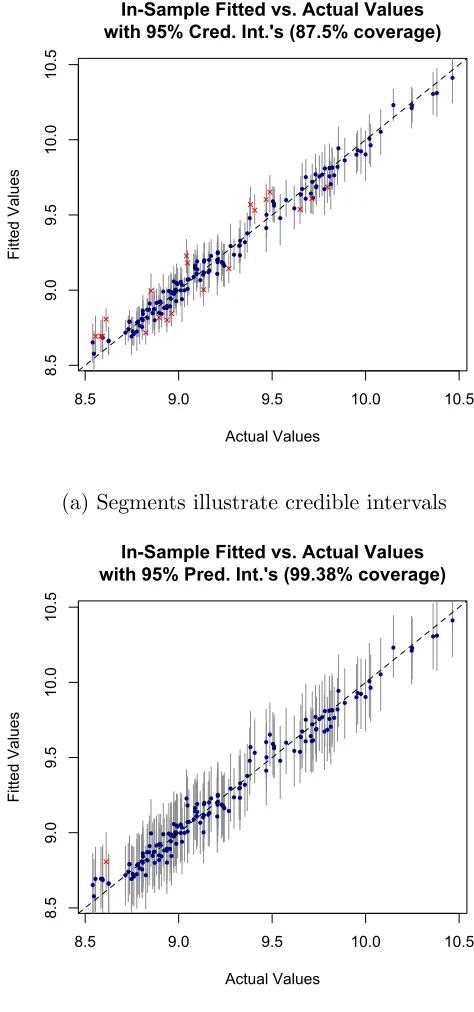
2.3.4 Credible intervals and prediction intervals . . . 38
2.3.5 Variable importance . . . 39
2.3.6 Variable effects . . . 39
2.3.7 Partial dependence . . . 44
2.3.8 Incorporating missing data . . . 45
2.3.9 Variable selection . . . 48
2.3.10 Informed prior information on covariates . . . 51
2.3.11 Interaction effect detection . . . 52
2.3.12 bartMachine Model Persistence Across R Sessions . . . 53
2.4 bartMachine Package Features for Classification . . . 55
2.5 Conclusion . . . 60
2.5.1 Forecasting “Bakeoff” . . . 60
2.5.2 Discussion . . . 61
3 Variable Selection for BART 62 3.1 Introduction . . . 63
3.2 Techniques for Variable Selection . . . 65
3.2.1 Linear Methods . . . 65
3.2.2 Tree-Based Methods . . . 66
3.3 Calibrating BARTOutput for Variable Selection . . . 67
3.3.1 BART Variable Inclusion Proportions . . . 69
3.3.2 Further Exploration of Null Simulation . . . 70
3.3.3 Variable Inclusion Proportions under Permuted Responses . . 74
3.3.4 Real Prior Information inBART-based Variable Selection . . . 79
3.4 Simulation Evaluation of BART-based Variable Selection . . . 80
3.4.1 Simulation Setting 1: Linear Relationship . . . 84
3.4.2 Simulation Setting 2: Nonlinear Relationship . . . 87
3.4.3 Simulation Setting 3: Linear Model with Informed Priors . . . 90
3.5 Application to Gene Regulation in Yeast . . . 93
3.6 Conclusion . . . 101
4 Incorporating Missingness into BART 104 4.1 Introduction . . . 104
4.2 Background . . . 106
4.2.1 A Framework for Missing Data in Statistical Learning . . . 106
4.2.2 Strategies for Incorporating Missing Data in Statistical Learning 110 4.2.3 Missing data in Binary Decision Trees . . . 112
4.3 Missing Incorporated in Attributes withinBART . . . 113
4.4 Generated Data Simulations . . . 116
4.4.1 A Simple pattern-mixture Model . . . 116
4.4.2 Selection Model Performance . . . 120
4.6 Discussion . . . 126
5 BART with Parametric Models of Heteroskedasticity 130 5.1 Introduction . . . 130
5.2 Bayesian Heteroskedastic Regression . . . 132
5.3 AugmentingBART to Incorporate Heteroskedasticity . . . 133
5.3.1 Priors and Likelihood . . . 135
5.3.2 Sampling from the Posterior . . . 136
5.4 Simulations . . . 139
5.4.1 Univariate Model . . . 139
5.4.2 Multivariate Model . . . 142
5.5 Real Data Examples . . . 145
5.5.1 Lidar Data . . . 145
5.5.2 Motorcycle Data . . . 145
5.6 Discussion . . . 148
6 Ensemble-of-Trees Algorithms in Criminology 150 6.1 Introduction . . . 151
6.2 Proper Criminal Justice Forecasting Comparisons . . . 154
6.2.1 Some Common-Sense Requirements for Fair Forecasting Com-parisons . . . 156
6.3 Some Conceptual Fundamentals . . . 159
6.3.1 The Basic Account . . . 159
6.3.2 Building in Differential Forecasting Error Costs . . . 163
6.3.3 Nonlinear Decision Boundaries . . . 165
6.3.4 Enter Machine Learning . . . 169
6.4 The Forecasting Contestants . . . 170
6.4.1 Logistic Regression with Asymmetric Costs . . . 171
6.4.2 Random Forests with Asymmetric Costs . . . 172
6.4.3 Asymmetric Costs in Stochastic Gradient Boosting . . . 173
6.4.4 A Simulation . . . 174
6.5 An Empirical Example . . . 179
6.5.1 Forecasting Arrests for Serious Crimes . . . 179
6.6 Conclusions . . . 182
7 Using Random Forests with Asymmetric Costs to Predict Hospital Readmissions 184 7.1 Background and Significance . . . 185
7.2 Objective . . . 188
7.3 Materials and Methods . . . 188
7.3.1 Setting . . . 188
7.3.2 Outcome Variables . . . 188
7.3.4 Random Forests with Asymmetric Costs . . . 189
7.3.5 Variable Selection . . . 190
7.3.6 Model Evaluation . . . 191
7.4 Results . . . 192
7.4.1 Descriptive Characteristics . . . 192
7.4.2 30-Day All-cause Readmissions Random Forests Model . . . . 193
7.4.3 7-Day Unplanned Readmissions Random Forests Model . . . . 196
7.5 Discussion . . . 197
7.6 Conclusion . . . 200
8 Bootstrapping for Stable Classification Trees 202 8.1 Introduction . . . 203
8.2 Modifying Classification Trees for Criminal Justice Settings . . . 205
8.2.1 Asymmetric Costs and Tuning . . . 207
8.2.2 Stability Analysis . . . 209
8.3 Data . . . 210
8.3.1 Variables . . . 211
8.4 Random Forest Results . . . 213
8.5 Classification Tree Results . . . 214
8.5.1 A Classification Tree Visualization . . . 216
8.5.2 Stability Analysis . . . 218
8.6 Conclusions . . . 225
9 Conclusion 227 A Appendices 229 A.1 Supplement for Chapter 1 . . . 229
A.1.1 Sampling New Trees . . . 229
A.1.2 Grow Proposal . . . 230
A.1.3 Prune Proposal . . . 235
A.1.4 Change . . . 236
A.2 Supplement for Chapter 3 . . . 240
A.2.1 Pseudo-code for Variable Selection Procedures . . . 240
A.3 Supplement for Chapter 5 . . . 244
A.4 Supplement for Chapter 8 . . . 253
List of Tables
2.1 BARTimplementation feature comparison . . . 24
2.2 Bakeoff of BayesTree,BART, and RF . . . 60
2.3 Runtimes forBayesTree, BART, and RF . . . 61
3.1 Nested variance decomposition of inclusion proportions variability . . 72
3.2 Distribution of prior influences values across 6026 genes . . . 99
4.1 Missing data mechanisms in statistical learning framework . . . 110
4.2 Missing data scenarios for Boston Housing data simulations . . . 124
6.1 Logistic regression confusion table using simulated test data. . . 177
6.2 Logistic regression with interaction confusion table using simulated test data. . . 178
6.3 Random forests confusion table using simulated test data. . . 179
6.4 Logistic regression test data confusion table for serious crime. . . 180
6.5 Random forests test data confusion table for serious crime. . . 181
6.6 Stochastic gradient boosting test data confusion table for serious crime. 181 7.1 University of Pennsylvania Health System study cohort characteristics 192 7.2 Incidence rates for 30-day all cause and 7-day readmissions . . . 193
8.1 RF confusion table for violent crime prediction . . . 213
List of Figures
1.1 Growing a classification tree . . . 6
2.1 Runtime comparisons forBART implementations . . . 27
2.2 Out-of-sample predictive performance by number of trees. . . 33
2.3 BARTmodel assumption checking plots . . . 36
2.4 BART convergence diagonstic plots . . . 37
2.5 Fitted versus actual values for automobile dataset . . . 40
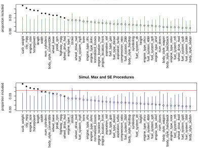
2.6 Average variable inclusion proportions for automobile data . . . 41
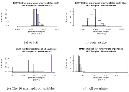
2.7 Tests of covariate importance . . . 43
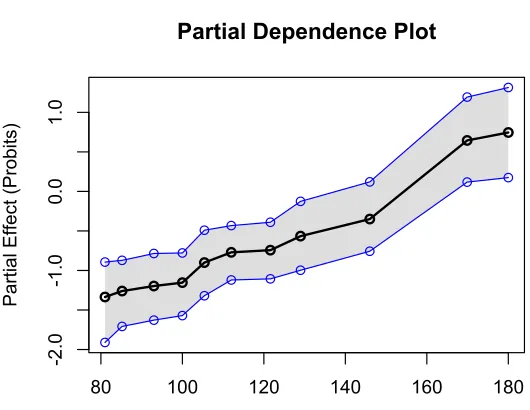
2.8 Partial dependence plots for automobile data . . . 46
2.9 Visualization of variable selection procedure . . . 50
2.10 Top interaction counts for Friedman function data . . . 54
2.11 Covariate importance test for Pima Indians data . . . 59
2.12 Partial dependence plot for predictor glu from Pima Indians data . . 59
3.1 Variable inclusion proportions in null setting . . . 71
3.2 Visualization of nested variance decomposition . . . 74
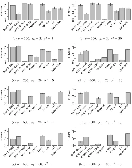
3.3 Top variable inclusion proportions for yeast geenYAL004W with selection 78 3.4 Average F1 scores by method for linear simulation setting . . . 86
3.5 Average F1 scores by method for nonlinear simulation setting . . . 89
3.6 Average F1 scores for different BART prior choices . . . 92
3.7 Distributions of number of predictors selected by method across 6026 genes . . . 97
3.8 Distributions of RMSE reduction per predictor by method across 6026 genes . . . 99
4.1 BART estimation of conditional means under different missing data
mechanisms . . . 118
4.2 BARTm versus complete-case analysis results . . . 123
4.3 Bakeoff results for Boston Housing Data . . . 127
5.1 BART’s andHBART’s posterior mean estimates . . . 140
5.2 Estimates of the conditional mean function f for HBART and BART . . 143
5.3 Distribution of out-of-sample RMSE forBART and HBART . . . 144
5.4 Posterior mean estimates for BARTand HBART(Lidar data) . . . 146
5.5 Posterior predictive intervals for many methods (motorcycle data) . . 147
6.1 Two linear decision boundaries in 2-dimensional predictor space . . . 160
6.2 Impact of asymmetric costs in 2-dimensional predictor space . . . 164
6.3 Linear and nonlinear 2D decision boundary . . . 165
6.4 Challenging classification surface for parametric models . . . 175
7.1 RF confusion matrix for 30-day readmissions on training data . . . 194
7.2 RF confusion matrix for 30-day readmissions on validation data . . . . 195
7.3 Variable importance plot for 30-day all-cause readmissions RF model . 195 7.4 RF confusion matrix for 7-day readmissions on training data . . . 197
7.5 RF confusion matrix for 7-day readmissions on validation data . . . . 198
7.6 Variable importance plot for 7-day unplanned readmissionsRF model 198 8.1 Classification tree for arrest for violent crime . . . 217
1
Introduction
1.1
Overview
Leo Breiman eloquently captures the motivation for and aim of statistical machine
learning in his 2001 Statistical Science paper:
“The approach is that nature produces data in a black box whose insides
are complex, mysterious, and, at least, partly unknowable. What is
ob-served is a set ofx0sthat go in and a subsequent set ofy0sthat come out.
The problem is to find an algorithm f(x) such that for future x in a test
set, f(x) will be a good predictor of y.”
For the past few decades, statisticians and computer scientists have sought to
uncover “nature’s black box” across a wide array of domains and applications, leading
to many novel algorithms and advancements in a field that today has come to be
known as “supervised learning.”
In particular, ensemble methods have gained much popularity in supervised
learn-ing problems, where the goal is to estimate this unknown function f from observed
combine them together in some fashion to produce a final model. In both theory and
practice, ensemble methods are often able to improve predictive performance relative
to the capabilities of the base algorithms that constitute the ensemble. Such findings
hold true for both regression and classification settings (Rokach, 2009).
We focus in particular on ensemble-of-trees procedures. These algorithms are
ma-chine learning techniques that use decision trees, such as Classification and Regression
Trees (CART, Breiman et al., 1984), as the base learner. As a standalone technique,
decision trees provide highly interpretable models that can effectively capture
interac-tion effects and nonlinearities (Chipman et al., 2010). Regarding predictive accuracy,
decision trees fare reasonably well; Breiman (2001b) states that decision trees rate
“a B on prediction.” More recent efforts in machine learning though have studied
the predictive performance of ensembles of decision trees. Such techniques include
random forests (RF, Breiman, 2001a), stochastic gradient boosting (SGB, Friedman,
2002), Bayesian Additive Regression Trees (BART, Chipman et al., 2010) and Dynamic
Trees (DT, Taddy et al., 2011). The aforementioned algorithms have achieved
supe-rior predictive accuracy across a wide array of domains and rank among the most
competitive techniques for supervised learning to date. In order to achieve strong
predictive performance, these models sacrifice a high degree of interpretability
associ-ated with the component decision trees. For example, Breiman (2001b) remarks that
RF “are A+ predictors...on interpretability, they rate an F.” Much work has been
done to improve the interpretability of such “black-box” algorithms, and some new
developments will be presented in this work.
The ensemble-of-trees methods can be divided into two distinct groups. The first
group contains the supervised learning procedures that are constructed in a purely
algorithmic fashion; there is no statistical model underlying the technique. RFandSGB
learning procedures that posit an underlying probability model. BART and DT, two
members of the second group, are both based on Bayesian probability models. In the
first component of this thesis, we develop methodological extensions for the models
in the second group, particularly forBART. In the second half of this thesis, we return
to the algorithmically-motivated procedures and explore applications in criminology
and healthcare where there are asymmetric costs associated with forecasting errors.
The remainder of this thesis is organized as follows. In the subsequent sections of
this chapter, we first reviewCARTas an example of how a decision tree is constructed.
We next briefly review RF andSGB, and then provide a a more extensive introduction
to BART. Each chapter following the introduction is adapted from a specific article
(cited at the end of each chapter) and modified for coherence within the overall thesis.
The next four chapters develop extensions for BART. Chapter 2 introduces
bartMachine, a new R package implementing BART for both robust research and
ap-plication, highlighting key performance and visualization features of the package.
Using the bartMachineimplementation as a computational engine, we then develop
a number of methodological innovations for BART. Chapter 3 develops a method for
principled nonparametric variable selection using BART. The approach relies on
ap-plying frequentist permutation testing ideas to output from a Bayesian model. We
additionally develop a means for incoporating informed prior information into the
variable selection and demonstrate the promise of our approach via an application
to inferring the genetic regulatory network in yeast. The third methodological
in-novation, discussed in Chapter 4, offers an approach for incorporating missing data
into BART in both the training and forecasting phases. The approach takes
advan-tage of the structure of decision trees and does not require any imputation. Finally,
Chapter 5 relaxes the assumption of homoskedasticity in the original BART model
BART.
Following the methodological innovations, Chapters 6-8 discuss applications of
ensemble-of-trees methods in classification problems where forecasting errors
associ-ated with each outcome class have asymmetric costs. Chapter 6 advocates for the
superiority of RF and SGB over traditional techniques such as logistic regression in
criminology applications with asymmetric forecasting costs. The exposition in the
chapter is largely didactic and meant to highlight the general merits of machine
learning methods over parametric modeling for prediction problems in criminology.
Continuing with the theme of asymmetric costs incorporated into ensemble-of-trees
models, we next switch the subject matter domain. Chapter 7 proposes RF models
for forecasts of unplanned hospital readmissions that rely on a large set of patient
covariates. The models herein are designed to be used in real-time upon patient
discharge and account for the asymmetric forecasting costs that health system
ad-ministrators face. Finally, we return to the criminology setting to explore a scenario
where traditional ensemble methods may not be available. Chapter 8 develops
pro-totype classification tree models that can be used in sentencing decisions for courts
where the technology to access more sophisticated procedures may not be available.
We develop an approach to generate trees with stable predictions by examining
classi-fication agreement across an ensemble of bootstrapped trees. Finally, Chater 9 offers
directions for future research and concludes.
1.2
Decision Trees
The basic building block for all ensemble-of-trees algorithms is the decision tree.
Although multiple versions of decision trees have been proposed in the literature,
understand the ensemble methods developed herein. The ensuing discussion draws
from Breiman et al. (1984) and Hastie et al. (2009).
At a high level, decision trees partition the observed data (or training data) into
subsets with similar values of the response. This is accomplished by exploiting the
predictors to create the greatest homogeneity between the observed outcomes and the
outcomes that the tree can project. Let y denote the response vector, which may be
continuous or categorical, and let x1,· · · ,xp denote the set ofppredictors as column vectors. With this notation, we can describe the general construction of aCART tree.
After introducing the algorithm, we will highlight key aspects of regression trees and
classification trees separately.
First, all of the observations begin in a single node known as the “root node.”
The data is the partitioned into two child nodes by considering “splitting rules” of
the form xj < c. Here, xj denotes the “splitting variable” (or “splitting attribute”) andcdenotes the “splitting value.” All observations satisfying the “splitting rule” are
sent to the left child node and the rest of the observations are sent to the right child
node. Using a greedy approach, all possible splitting rules that can be created from
the observed data are evaluated and the rule that minimizes some statistical criterion
is chosen. Once a split is selected, the observations are moved to their respective
nodes and the above process is repeated for each of the two child nodes. Such split
construction proceeds in a recursive fashion until a stopping rule is satisfied. Examples
of common stopping rules include a maximum depth for which a tree is allowed to
grow, a constraint on the minimum number of observations in a node, or a required
reduction in the value of the statistical criterion selected. Nodes which no longer split
are labelled “terminal nodes.” The construction of a CART tree is completed once all
nodes are labelled as terminal. Note that in some cases, the nodes are removed
CART pruning as it is generally not applicable to the understanding of the ensemble
methods we discuss.
After tree construction, fitted values are assigned to each terminal node based
on the observations that land in that node. As will be shown, the fitted values
will be an average of response values for regression trees and the majority class (or
plurality class for multi-class problems) in the node for classification trees. Forecasts
for observations with an unknown response can be obtained by “dropping” the cases
down the tree and following the path implied by the splitting rules. The forecast
assigned to the observation is the fitted value associated with the terminal node in
which the observation lands.
Figure 1.1 shows two steps in the growth of a classification tree for response y
with levels “0” and “1” and predictors x1 and x2. Terminal nodes are assigned the
majority class as evidenced by the proportion of outcome classes given in the terminal
nodes.
With the general CART algorithm in place, we now highlight the specifics of
clas-sification trees and regression trees.
x2 < 0.83
0 .62 .38
1 .07 .93
(a) Depth 1 classification tree
x2 < 0.83
x1 < 0.13
x2 < 0.26
0 1.00 .00
0 .74 .26
1 .49 .51
1 .07 .93
(b) Depth 2 classification tree
1.2.1
Classification Trees
Classification trees are employed for data with categorical response variables. Suppose
there are K distinct classes for the response in the training data. For the mth node
in the tree, let Pm represent the set of observations in node m of size Nm. One can
compute
ˆ
pmk = 1
Nm X
i∈Pm
I(yi =k) (1.1)
which is the empirical proportion of observations belonging to classk in nodem. ˆpmk
is then used to define the statistical criterion used to determine the optimal splitting
rule at each step in growing classification trees. This criterion acts to minimize
within-node homogeneity of class labels and are often called “impurity functions.” Breiman
et al. (1984) proposes three commonly impurity functions:
Misclassification error : 1
Nm X
i∈Pm
I(yi 6=hatcm) (1.2)
Gini index : X
k6=k0 ˆ
pmkpˆmk0 (1.3)
Cross-entropy : −
K X
k=1
ˆ
pmklog (ˆpmk) (1.4)
In practice, the Gini index or cross-entropy are more commonly employed as they are
smooth functions and hence more amenable to optimization. These criteria are also
more sensitive to changes in the node probabilities compared to the misclassification
error.
Letting φ denote an impurity function evaluated on the observations in node m,
∆ (s, m) = φ(m)− 1
NmL
φ(mL)− 1
NmR
φ(mR) (1.5)
where mL and mR denote the left and right child nodes resulting from splitting rule
s on node m. The splitting rule that maximizes ∆ (s, m) across all available rules is
selected and the tree is partitioned.
Once the classification tree has been fully grown, fitted values for terminal nodes
are often assigned by taking the plurality class in the node. Letting ˆcm denoted the
fitted value for a (terminal) node m, we have
ˆ
cm = argmax
k ˆ
pmk. (1.6)
Note that the assignment above operates under the assumption of symmetric costs
for misclassification errors. We will introduce asymmetric misclassification costs and
the appropriate modifications to theCART algorithm in Chapter 8.
1.2.2
Regression Trees
Regression trees are employed for data with continuous response variables. For
regression trees, the impurity function used for CART is the sum of square errors
P
i∈Pm(yi −y¯m)
2
where ¯ym is the average of the observations in node m. The
split-ting rule s that maximizes ∆ (s, m) for node m is selected at each partitioning step.
Terminal node fitted values in regression trees are given by the average value of
ˆ
cm = 1
Nm X
i∈Pm
yi. (1.7)
1.3
Algorithmic Ensemble-of-trees Techniques
Two popular ensemble-of-trees techniques, RF and SGB traditionally use CART trees
as the basic building blocks of their ensembles. The trees serve as the base learners
within the algorithm and the output of each tree is combined to create a final fitted
value or forecast. RF and SGB use the CART trees in substantially different fashions
and we review each algorithm in the subsequent sections. The discussion forRF draws
from Breiman (2001a) and Hastie et al. (2009, chapter 15), and the discussion for
SGB draws upon Friedman (2002) and Hastie et al. (2009, chapter 10).
1.3.1
Random Forests
RF builds upon a method known as “bootstrap aggregation,” or “bagging” (Breiman,
1996), in which multiple versions of some base learner are independently constructed
on different bootstrapped samples of the data. In bagging, the forecasts from each of
the learners is then aggregated, often via averaging for continuous responses or
plural-ity vote for categorical responses. When grown sufficiently deep, trees are especially
good candidates for bagging as they are considered to be low-bias, high variance
learn-ers. Aggregrating across multiple instances can work to lower variance and reduce
generalization error.
RF takes bagging one step further in an effort to further reduce variance. The
evaluating a subset of predictors rather than all predictors. By choosing m∗ ≤ p
predictors, an additional source of randomness is introduced into the tree-growing
process. This randomness decorrelates the decision trees across the ensemble (at the
expense of a slight increase in the individual variance of each tree), which can further
reduce the variance of the aggregated ensemble.
RF contains two important tuning parameters. The first is the number of decision
trees to grow in the ensemble. Typically, no more than 500 decision trees are needed
for the performance of RF to stabilize and the procedure does not overfit the data as
the number of trees grows larger. The second tuning parameter is m∗, the number
of predictors to evaluate at each split. For regression problems, p/3 is recommended
and for classification problems,√pis the commonly used default. Empirical evidence
suggests that RF is fairly robust to choices of these tuning parameters. For certain
applications, additionally tuning the minimum number of observations required to
split a node may also be useful. Algorithm 1 provides the pseudocode for the default
RF algorithm.
Algorithm 1 Random Forests
1. Forb = 1 to B:
(a) Draw a bootstrap sampleX∗ of size N from the training data
(b) Grow a decision treeTb to the data X∗ by doing the following recursively until the minimum node sizenmin is reached:
i. Select m∗ of the pvariables
ii. Pick the best split from them∗ variables and partition 2. Output the ensemble{Tb}Bb
Classification: Let ˆCb(x∗) be the predicted class for x∗ tree Tb. Then ˆCrfB(x
∗) =
plurality vote{Cˆb(x∗)}B1.
Regression: Let ˆfb(x∗) be the predicted value from tree Tb. Then ˆfrfB(x∗) = 1
B B P i=1
ˆ
fb(x∗).
observation down each decision tree as described in the above algorithm. However,
there is often interest in obtaining fitted values for the training data. Such estimates
can be obtained via “out-of-bag” (OOB) estimates. OOB estimates are computed
by obtaining the forecasts for observations in the training data on decision trees for
which the observations were not used to construct the tree. This implies that such
observations were not selected in the bootstrap sample X∗ and hence are referred to as out-of-bag for such trees. For each observation, the set of forecasts from each tree
is then aggregated to produce a single fitted value. Given that OOB estimates are
obtained from trees where the observation did not contribute to tree construction,
the estimates are often a good proxy for true out-of-sample performance. We will
make extensive use of this fact in Chapters 6-8 to tune theRF models for asymmetric
costs of forecasting errors.
Throughout this work, we use the RF implementation provided in the R package
randomForest (Liaw and Wiener, 2002).
1.3.2
Stochastic Gradient Boosting
In constrat toRF which aggregates a collection of independent base learners,SGB
op-erates on a set of learners in a stepwise fashion. SGB proceeds by taking a pass
through the data, constructing a base learner, and then reweighting observations
that were more difficult to correctly classify. While there are numerous flavors of
boosting that each result in different reweighting schemes for the data, SGB operates
on the negative partial derivatives of the loss function at each training observation.
These partial derivatives are often referred to as “pseudo-residuals”. A regression tree
is then grown to the pseudo-residuals, thereby using partitions of predictor space to
by computing the addition to the current fit that minimizes the loss function. The
current fitted values are then updated by adding the computed terminal node values
to the existing fitted values for each observation.
Friedman (2001) originally proposed the above algorithm under the name
“gra-dient boosting.” In this implementation, each regression tree was constructed on
the entire set of training data. Friedman (2002) modified the algorithm to select a
random bootstrap sample of training observations for growing each regression tree,
resulting in the name stochastic gradient boosting. This subsampling step results in variance reduction, which improves performance through lower generalization error.
SGB contains a number of important tuning parameters as well. The first is the
“learning rate”ν. The update to the current fitted values are shrunk byν to control
how quickly the algorithm descends down the gradient of the loss function. The
learning rate provides regularization through shrinkage. The second parameter is the
number of boosting iterations T. It is well-known that boosting algorithms overfit
the data as the number of iterations grows and too many iterations can result in poor
generalization error. There is a tradeoff between ν and T, however. Lower values of
ν allow for more iterations without too much overfitting. However, this relationship
between ν and T is not direct, and hence Ridgeway (2006) recommends choosing
a small value of ν to not descend the gradient too quickly and then select T via
cross-validation. The third important tuning parameter is the depth to which the
regression trees are grown. Deeper trees allow for higher order interaction effects.
Depths between 2-6 work well in practice (Ridgeway, 2006) and can be chosen via
cross-validation.
Algorithm 2 provides the pseudocode for SGB for general loss functions.
Com-monly used loss functions include squared error loss or absolute loss for continuous
Implementations of loss functions for Poisson-distributed, multinomial, and censored
outcomes have been developed as well. The reader is referred to Ridgeway (2006) for
a more complete discussion of available loss functions.
Algorithm 2 Stochastic Gradient Boosting
1. Initialize f0(x) = arg min γ Pn
i=1L(yi, γ)
2. Fort = 1 to T:
(a) Draw a bootstrap sampleX∗ of size N from the training data:
(b) Fori= 1,2, ..., N compute:
rim =− n
∂L(yi,f(xi))
∂f(xi)
o f=ft−1
i∈X∗
(c) Fit a regression tree to the rit yielding terminal nodesRjt, j = 1, ..., Jt (d) Forj = 1,2, , ..., Jt compute:
γjt = argmin ν
P xi∈Rjt
L(yi, ft−1(x) +γ)
(e) Updateft(x) = ft−1+ν·PJj=1t γjtI(x∈Rjt) 3. Output ˆf(x) =fT(x)
Throughout this work, we use theSGB implementation provided in theRpackagegbm
(Ridgeway, 2006).
1.4
Bayesian Additive Regression Trees
BART differs fromRFandSGB by relying on an underlying probability model to
gener-ate estimgener-ates of some unknown functionf rather than a purely algorithmic approach.
BART uses a Bayesian probability model to generate a posterior distribution forf(x).
In this section, we extensively develop the BART model. The ensuing development is
adapted from Kapelner and Bleich (2015) and also draws from Chipman et al. (2010).
BART can be considered a sum-of-trees ensemble. While single decision trees are
effective for capturing nonlinearities and interaction effects inf, a sum-of-trees model
allows for better fitting of additive components in f. Specifically, the BART model
Y =f(X) +E ≈il1(X) +il2(X) +. . .+ilm(X) +E, E ∼ Nn 0, σ2In
(1.8)
where Y is the n×1 random vector of responses, X is the n×p design matrix (the
predictors column-joined) and E is the n×1 vector of noise. Here we have mdistinct
regression trees, each composed of a tree structure, denoted byi, and the parameters
at the terminal nodes (also called leaves), denoted by l. The two together, denoted
as il represents an entire tree with both its structure and set of leaf parameters. The structure of a given tree it includes all of the splitting rules, allowing one to
specify how any observation traverses down the tree. We denote the parameters for
the leaves of the tree as lt= {µt,1, µt,2, . . . , µtbt} where bt is the number of terminal
nodes for a given tree. An observation’s predicted value is the sum of the m leaf
values arrived at by traversing down all m trees.
As a Bayesian model,BART consists of a set of priors for the structure and the leaf
parameters and a likelihood for data in the terminal nodes. The aim of the priors is
to provide regularization, preventing any single regression tree from dominating the
total fit. We first provide an overview of the priors forBART and likelihood and then
discuss how draws from the posterior distribution are made.
1.4.1
Priors and likelihood
The prior for the BART model has three components: (1) the tree structure itself, (2)
the leaf parameters given the tree structure, and (3) the error variance σ2 which is
P
il1, . . . ,ilm, σ2 = "
Y
t
P
ilt
#
P σ2 (1.9)
= " Y t P
lt | it P it #
P σ2 (1.10)
= " Y t Y ` P
µt,` | it P it #
P σ2 (1.11)
where the last equality follows from an additional assumption of conditional
indepen-dence of the leaf parameters given the tree’s structure.
We first describe Pit
, the component of the prior which affects the locations
of nodes within the tree. Node depth is defined as distance from the root. Thus,
the root itself has depth 0, its first child node has depth 1, etc. Nodes at depth d
are nonterminal with prior probability α(1 +d)−β where α ∈ (0,1) and β ∈ [0,∞].
This component of the tree structure prior has the ability to enforce shallow tree
structures, thereby limiting complexity of any single tree and resulting in more model
regularization. Default values for these hyperparameters of α = 0.95 and β = 2 are
recommended by Chipman et al. (2010).
For nonterminal nodes, splitting rules occur in two parts. First, a predictor is
randomly selected to serve as the splitting variable. In the original formulation, each
available predictor is equally likely to be chosen from a discrete uniform distribution,
and hence each variable is selected with probability 1/p. This is relaxed in our
im-plementation to allow for a generalized Bernoulli distribution where the user specifies
p1, p2, . . . , pp (such that Pp
j=1pj = 1), where pj denotes the probability of the jth
variable being selected a priori. This more general prior will be developed further in Chapter 3. Additionally, note that “structural zeroes,” variables that do not have
al-gorithm (see Appendix A.1.2 for details). Once the splitting variable is chosen, the
splitting value is chosen from the multiset (the non-unique set) of available values at
the node via the discrete uniform distribution.
We now describe the prior component Plt |it
which controls the leaf
param-eters. Given a tree with a set of terminal nodes, each terminal node (or leaf) has a
continuous parameter (the leaf parameter) representing the “best guess” of the
re-sponse in this partition of predictor space. This parameter is the fitted value assigned
to any observation that lands in that node. The prior on each of the leaf parameters
is given as: µ` iid
∼ N µµ/m, σ2µ
. The expectation, µµ, is picked to be at the range
center, (ymin+ymax)/2.
The variance hyperparameter σ2
µ is empirically chosen so that the range center
plus or minus k = 2 variances cover 95% of the provided response values in the
training set (where k = 2 corresponding to 95% coverage is only by default and
can be customized). Thus, since there are m trees, we then choose σµ such that
mµµ − k
√
mσµ = ymin and mµµ +k
√
mσµ = ymax. The aim of this prior is to
provide model regularization by shrinking the leaf parameters towards the center of
the distribution of the response. The larger the value of k, the smaller the value of
σ2
µ, resulting in more model regularization.
The final prior is on the error variance and is σ2 ∼ InvGamma (ν/2, νλ/2). λ
is determined from the data so that there is a q = 90% a priori chance (by default)
that the BART model will improve upon the root mean square error (RMSE) from
an ordinary least squares regression. Therefore, the majority of the prior probability
mass lies below the RMSE from least squares regression. Additionally, this prior
limits the probability mass placed on small values ofσ2 to prevent overfitting. Thus,
the higher the value of q, the larger the values of the sampledσ2’s, resulting in more
Note that the adjustable hyperparameters are α, β, k, ν and q. Additionally,
m, the number of trees, must be chosen. Default values generally provide good
performance, but optimal tuning can be achieved automatically via cross-validation.
Along with a set of priors,BART specifies the likelihood of responses in the terminal
nodes. They are assumed a priori normal with the mean being the “best guess” in the
leaf at the moment (i.e. in the current Markov chain Monte Carlo (MCMC) iteration)
and variance being the best guess of the variance at the moment, y` ∼ N(µ`, σ2).
1.4.2
Posterior distribution and prediction
A Metropolis-within-Gibbs sampler (Geman and Geman, 1984; Hastings, 1970) is
employed to generate draws from the posterior distribution of P(il1 , . . . ,i
l
m, σ2 | y). A key feature of this sampler for BART is to employ a form of “Bayesian backfitting”
(Hastie and Tibshirani, 2000) where the jth tree is fit iteratively, holding all other
m−1 trees constant by exposing only the residual response that remains unfitted:
R−j :=y− X
t6=j
ilt (X). (1.12)
The sampler,
1 : i1 | R−1, σ2 (1.13)
2 : l1 | i1,R−1, σ2
3 : i2 | R−2, σ2
4 : l2 | i2,R−2, σ2 ..
2m−1 : im |R−m, σ2
2m: lm | im,R−m, σ2
2m+ 1 : σ2 |i1,l1, . . . ,im,lm,E,
proceeds by first proposing a change to the first tree’s structurei which are accepted
or rejected via a Metropolis-Hastings step. Note that sampling from the posterior of
the tree structure does not depend on the leaf parameters, as they can be analytically
integrated out of the computation (see Appendix A.1.2). Given the tree structure,
samples from the posterior of thebleaf parametersl1 :={µ1, . . . , µb}are then drawn.
This procedure progresses iteratively for each tree, using the updated set of partial
residuals R−j. Finally, conditional on the updated set of tree structures and leaf parameters, a draw from the posterior ofσ2 is made based on the full model residuals
E :=y−Pmt=1ilt (X).
Within a given terminal node, since both the prior and likelihood are normally
distributed, the posterior of each of the leaf parameters inlis conjugate normal with
its mean being a weighted combination of the likelihood and prior parameters (lines
2, 4, . . . ,2m in Equation set 1.13). Due to the normal-inverse-gamma conjugacy, the
posterior of σ2 is inverse gamma as well (line 2m+ 1 in Equation set 1.13). The
complete expressions for these posteriors can be found in Gelman et al. (2004).
Lines 1, 3, . . . , 2m−1 in Equation set 1.13 rely on Metropolis-Hastings draws from
the posterior of the tree distributions. These involve introducing small perturbations
to the tree structure: growing a terminal node by adding two child nodes, pruning
two child nodes (rendering their parent node terminal), or changing a split rule. We
denote the three possible tree alterations as: GROW, PRUNE, and CHANGE.1 The
1In the original formulation, Chipman et al. (2010) include an additional alteration called SWAP.
mathematics associated with the Metropolis-Hastings step are tedious. Appendix A.1
contains the explicit calculations. Once again, over many MCMC iterations, trees
evolve to capture the fit left currently unexplained.
All 2m+ 1 steps represent a single Gibbs iteration. Empirical work suggests that no more than 1,000 iterations are needed as “burn-in,” although diagnostics can be
used to assess the MCMC chain (see Chapter 2). An additional 1,000 iterations are
usually sufficient to serve as draws from the posterior for f(x). A single predicted value ˆf(x) can be obtained by taking the average of the posterior values and a quantile estimate can be obtained by computing the appropriate quantile of the posterior
values. Additional features of the posterior distribution will be discussed in Chapter 2.
1.4.3
BART
for classification
BART can easily be modified to handle classification problems for categorical response
variables. In Chipman et al. (2010), only binary outcomes were explored but recent
work has extended BART to the multiclass problem (Kindo et al., 2013). All work
herein focuses on the binary classification problem and we limit the discussion to
that scenario.
For the binary classification problem (coded with outcomes “0” and “1”), we
assume a probit model,
P(Y = 1 | X) = Φ
il1 (X) +il2(X) +. . .+ilm(X)
, (1.14)
where Φ denotes the cumulative distribution function of the standard normal
dis-tribution. In this formulation, the sum-of-trees model serves as an estimate of the
estimate of Y = 1.
In the classification setting, the prior on σ2 is not needed as the model assumes
σ2 = 1. The prior on the tree structure remains the same as in the regression setting
and a few minor modifications are required for the prior on the leaf parameters.
Sampling from the posterior distribution is again obtained via Gibbs sampling with
a Metropolis-Hastings step outlined in Section 1.4.2. Following the data augmentation
approach of Albert and Chib (1993), an additional vector of latent variables Z is
introduced into the Gibbs sampler. Then, a new step is created in the Gibbs sampler
where draws of Z|y are obtained by conditioning on the sum-of-trees model:
Zi |yi = 1 ∼ maxN X
t
ilt (X),1 !
, 0 and (1.15)
Zi |yi = 0 ∼ min (
N X
t
ilt (X),1 !
, 0 )
. (1.16)
Next, Z is used as the response vector instead ofy in all steps of Equation 1.13. Upon obtaining a sufficient number of samples from the posterior, inferences can
be made using the the posterior distribution of conditional probabilities and
classifica-tion can be undertaken by applying a threshold to the averages (or another summary)
of these posterior probabilities.
1.4.4
BART
Implementation
BART was implemented by the algorithm’s original authors in theRpackageBayesTree.
Chapter 2 develops a new novelRimplementation forBART,bartMachine. Unless
2
Bayesian Additive Regression Trees Implementation
Abstract
We present a new package inRimplementingBART. The package introduces many new
features for data analysis usingBART such as variable selection, interaction detection,
model diagnostic plots, incorporation of missing data and the ability to save trees
for future prediction. It is significantly faster than the current R implementation,
parallelized, and capable of handling both large sample sizes and high-dimensional
data.
2.1
Introduction
The initial implementation of BART was provided by Chipman et al. (2010) as a
supplement to the original work. The algorithm was developed with a C++
en-gine for constructing the ensemble with the output linked to R to allow for effective
data analysis. This implementation is available on CRAN in the packageBayesTree.
BayesTree, however, provides limited capabilities for a data analyst and lacks features
we develop a novel implementation of BART that draws inspiration from BayesTree,
but also attempts to remedy a number of its shortcomings in order to provide a more
broadly applicable BART toolbox to the statistics and machine learning communities.
The R package for our implementation,bartMachine, is available from the
Compre-hensiveRArchive Network athttp://CRAN.R-project.org/package=bartMachine.
We first highlight some key differences acrossBART implementations in Section 2.1.1
and then devote the rest of the chapter to eludicating the features of bartMachine.
In Section 2.2 we provide a general introduction to the package, highlighting the
novel features. Section 2.3 provides step-by-step examples of the regression
capabil-ities and Section 2.4 introduces additional step-by-step examples of features unique
to classification problems. We conclude in Section 2.5.
2.1.1
Comparison of
BART
Implementations
The goal of bartMachineis to provide a fast, easy-to-use, visualization-rich machine
learning package forRusers. In developingbartMachine, we explored otherBART
im-plementations and attempted to understand both the positives and negatives of each
implementation of the algorithm.
One of the most critical drawbacks of BayesTree is its lack of a standalone
predict function. Test data must be provided as an argument during the
train-ing phase of the model. Hence it is impossible to generate forecasts on future data
without re-fitting with the entire model. Since the run time is not trivial,
forecast-ing becomes an arduous exercise. A significantly faster implementation of BART that
contains master-slave parallelization was introduced in Pratola et al. (2013), but this
is only available as standalone C++ source code and not integrated with R.
response values to incorporate BART into a larger Bayesian model. dbarts relies on
BayesTree as its BART engine.
Our implementation of BART is in Java and is integrated into R via rJava
(Ur-banek, 2011). From a runtime perspective, our algorithm is significantly faster than
BayesTree and is parallelized, allowing computation on as many cores as desired.
Not only is the model construction itself parallelized, but the additional features such
as prediction, variable selection, and many others can be divided across cores as well.
We also include a variety of expanded and additional features. We implement the
ability to save trees in memory and provide convenience functions for prediction on
test data as well as the ability to save models across Rsessions. We also include
plot-ting functions for both posterior credible and predictive intervals and plots for visually
inspecting the convergence of BART ’s MCMC chain. We expand variable importance
exploration to include permutation tests and interaction detection. We implement
re-cently developed features for BART including a formal approach to variable selection
and the ability to incorporate prior information for covariates (Chapter 3). We also
implement a new strategy to incorporate missing data during training and handle
missingness during prediction without imputation (Chapter 4). Table 2.1 emphasizes
the differences in features between bartMachine and BayesTree, the two existing R
implementations of BART.
2.2
The
bartMachine
package
The package bartMachine provides a novel implementation of BART in R. The
algo-rithm is substantially faster than the currentRpackageBayesTreeand our
implemen-tation is parallelized at the MCMC iteration level during prediction. Additionally,
Feature bartMachine BayesTree
Implementation Language Java C++
External Predict Function Yes No
Model Persistence Across Sessions Yes No
Parallelization Yes No
Native Missing Data Mechanism Yes No
Built-in Cross-Validation Yes No
Variable Importance Statistical Tests Exploratory
Tree Proposal Types 3 Types 4 Types
Partial Dependence Plots Yes Yes
Convergence Plots Assess trees and σ2 Assess σ2
Model Diagnostics Yes No
Incorporation into Larger Model No Through dbarts
Table 2.1: Comparison of features between bartMachineand BayesTree.
to persist throughout theRsession, allowing for prediction and other calls to the trees
without having to re-run the Gibbs sampler (a limitation in the current BayesTree
implementation). ThebartMachineobject can be serialized, thereby persisting across
R sessions as well (a feature discussed in Section 2.3.12). Since our implementation
is different from BayesTree, we provide a predictive accuracy “bakeoff” on different
datasets in Section 2.5.1 which illustrates that the two exhibit similar performance.
2.2.1
Speed improvements and parallelization
We make a number of significant speed improvements over the original BayesTree
implementation.
First, bartMachine is fully parallelized (with the number of cores customizable)
during model creation, prediction, and many of the other features. During model
creation, we chose to parallelize by creating one independent Gibbs chain per core.
Thus, if we employ the default 250 burn-in samples and 1,000 post burn-in samples
post burn-in samples. The final model will aggregate the four post burn-in chains
for the four cores yielding the desired 1,000 total burn-in samples. This has the
drawback of effectively running the burn-in serially (which suffers from Amdahl’s
Law), but has the added benefit of reducing auto-correlation of the sum-of-trees
samples in the posterior samples since the chains are independent which may provide
greater predictive performance. Parallelization at the level of likelihood calculations
is left for a future release as we were unable to address the costs of thread overhead.
Parallelization for prediction and other features scale linearly in the number of cores
without Amdahl’s diminishing returns.
Additionally, we take advantage of a number of additional computational
short-cuts:
1. Computing the unfitted responses for each tree (Equation 1.12) can be
accom-plished by keeping a running vector and making entry-wise updates as the Gibbs
sampler (Equation 1.13) progresses from step 1 to 2m. Additionally, during theσ2
sampling (step 2m+ 1), the residuals do not have to be computed by traversing
the data down all the trees.
2. Each node caches its acceptable variables for split rules and the acceptable unique
split values so they do not need to be calculated at each tree sampling step. Recall
from the discussion concerning uniform splitting rules in Section 1.4.1 that
ac-ceptable predictors and values change based on the data available at an arbitrary
location in the tree structure. This speed enhancement, which we call memcache
comes at the expense of memory and may cause issues for large data sets. We
include a toggle in our implementation defaulted to “on.”
3. Careful calculations in Appendix A.1 eliminate many unnecessary computations.
re-sponses and no longer require computing the sum of the rere-sponses squared.
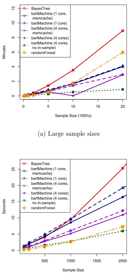
Figure 2.1 displays model creation speeds for different values ofnon a linear
regres-sion model withp= 20, normally distributed covariates,β1, . . . , β20 iid
∼ U (−1, 1), and
standard normal noise. Note that we do not vary p as it was already shown in
Chip-man et al. (2010) that BART’s computation time is largely unaffected by the
dimen-sionality of the problem. We include results forBARTusing BayesTree,bartMachine
with one core,bartMachinewith four cores having thememcache option both on and
off, and bartMachine with four cores, memcache off, and computation of in-sample
statistics off (all with m= 50 trees). The in-sample statistics that are computed by
default are in-sample predictions (ˆy), residuals (e:=y−yˆ),L1 error which is defined as Pntrain
i=1 |ei|, L2 error which is defined as
Pntrain
i=1 e 2
i, pseudo-R2 which is defined as
1−L2/(Pntrain
i=1 (yi−y¯) 2
) and RMSE which is defined as pL2/ntrain. We also
in-clude random forests model creation times via the packagerandomForest(Liaw and
Wiener, 2002) with its default settings.
We first note that Figure 2.1a demonstrates that thebartMachinemodel creation
runtime is approximately linear in n (without in-sample statistics computed). There
is about a 30% speed-up when using four cores instead of one. The memcache
en-hancement should be turned off only with sample sizes larger thann = 20,000 (data
unshown). Noteworthy is the 50% reduction in time of constructing the model when
not computing in-sample statistics. In-sample statistics are computed by default
be-cause the user generally wishes to see them. Also, for the purposes of this comparison,
BayesTree models compute the in-sample statistics by necessity since the trees are
not saved. The randomForest implementation becomes slower just after n = 1,000
due to its reliance on greedy exhaustive search at each node.
Figure 2.1b displays results for smaller sample sizes (n ≤ 2,000) that are often
0 5 10 15 20
0
2
4
6
8
10
12
Sample Size (1000's)
Mi
nu
te
s
BayesTree bartMachine (1 core,
memcache) bartMachine (1 core)
bartMachine (4 cores,
memcache) bartMachine (4 cores)
bartMachine (4 cores,
no in-sample)
randomForest
(a) Large sample sizes
500 1000 1500 2000
0
5
10
15
20
25
Sample Size
Se
co
nd
s
BayesTree bartMachine (1 core,
memcache) bartMachine (1 core)
bartMachine (4 cores,
memcache) bartMachine (4 cores)
bartMachine (4 cores,
no in-sample)
randomForest
(b) Small sample sizes
Figure 2.1: Model creation times as a function of sample size for a number of settings
of bartMachine,BayesTreeandrandomForest. Simulations were run on a quad-core
3.4GHz Intel i5 desktop with 24GB of RAM running the Windows 7 64bit operating
10% speed improvement. Thus, if memory is an issue, it can be turned off with little
performance degradation.
2.2.2
Implementation of Tree Alterations
Additionally, recall from Section 1.4.2, that there are 4 possible proposals for altering
the trees in BART originally proposed by Chipman et al. (2010): GROW, PRUNE,
CHANGE, and SWAP. bartMachine does not implement SWAP due to
complexi-ties that arise in implementation. Additionally, Pratola et al. (2013) argue that a
CHANGE step is unnecessary for sufficient mixing of the Gibbs sampler. While we
too observed this to be true for estimates of the posterior means, we found that
omit-ting CHANGE can negatively impact the variable inclusion proportions (the feature
introduced in Section 2.3.5). As a result, we implement a modified CHANGE step
where we only propose new splits for nodes that are singly internal (versus the original
proposal of changing any splitting rule in a tree). These are nodes where both
chil-dren nodes are terminal nodes (details are given in Appendix A.1.4). After a singly
internal node is selected we (1) select a new split attribute from the set of available
predictors and (2) select a new split value from the multiset of available values (these
two uniform splitting rules were explained in detail previously). We emphasize that
the CHANGE step does not alter tree structure.
2.2.3
Implementation of Research Features
The current stable release of bartMachineavailable on CRAN implements the
vari-able selection and informed prior procedures introduced in Chapter 3 and the method
for natively handling missing data proposed in Chapter 4. An experimental version
Chapter 5. Future work will involve incorporating this last feature into the package
available on CRAN.
2.3
bartMachine Package Features for Regression
We illustrate the package features by using both real and simulated data, focusing
first on regression problems.
2.3.1
Computing parameters
We first set some computing parameters. In this exploration, we allow up to 5GB of
RAM for the Java heap2 and we set the number of computing cores available for use
to 4.
R> options(java.parameters = "-Xmx5000m")
R> library("bartMachine")
R> set_bart_machine_num_cores(4)
bartMachine now using 4 cores.
The following Sections 2.3.2 – 2.3.9 use a dataset obtained from UCI repository
(Bache and Lichman, 2013). The n= 201 observations are automobiles and the goal
is to predict each automobile’s price from 25 features (15 continuous and 10 nominal),
first explored by Kibler et al. (1989).3 This dataset also contains missing data. We
omit missing data for now (41 observations that will later be retained in Section 2.3.8)
2Note that the maximum amount of memory can be set only once at the beginning of the
R
session (a limitation of rJava since only one Java Virtual Machine can be initiated perRsession), but the number of cores can be respecified at any time.
3We first preprocess the data. We first drop one of the nominal predictors (car company) due
and we create a variable for the design matrix X and the response y. The following code loads the data.
R> data(automobile)
R> automobile <- na.omit(automobile)
R> y <- automobile$log_price
R> X <- automobile; X$log_price <- NULL
2.3.2
Model building
We are now ready to construct a bartMachinemodel. The default hyperparameters
generally follow the recommendations of Chipman et al. (2010) and provide a
ready-to-use algorithm for many data problems. Our hyperparameter settings arem = 50,4
α = 0.95, β = 2, k = 2, q = 0.9, ν = 3, and probabilities of the GROW / PRUNE
/ CHANGE steps is 28% / 28% /44%. We retain the default number of burn-in
Gibbs samples (250) as well as the default number of post-burn-in samples (1,000).
In the default mode, the covariates are equally importanta priori. Other parameters and their defaults can be found in the package’s online manual. Below is a default
bartMachine model. Here, X denotes automobile attributes and y denotes the log
price of the automobile.
R> bart_machine <- bartMachine(X, y)
Building bartMachine for regression ...
evaluating in sample data...done
4In contrast to Chipman et al. (2010), we recommend this default as a good starting point
If one wishes to see more information about the individual iterations of the Gibbs
sampler of Equation 5.5, the flag verbose can be set to “TRUE.” One can see more
debug information from theJavaprogram by setting the flagdebug logto TRUE and
the program will print to unnamed.log in the current working directory. In the
fol-lowing code segment, we inspect the model object to query its in-sample performance
and to be reminded of the input data and model hyperparameters.
R> bart_machine
bartMachine v1.1.1 for regression
training data n = 160 and p = 41
built in 1.7 secs on 4 cores, 50 trees, 250 burn-in
and 1000 post. samples
sigsq est for y beforehand: 0.014
avg sigsq estimate after burn-in: 0.00794
in-sample statistics:
L1 = 8.01
L2 = 0.65
rmse = 0.06
Pseudo-Rsq = 0.979
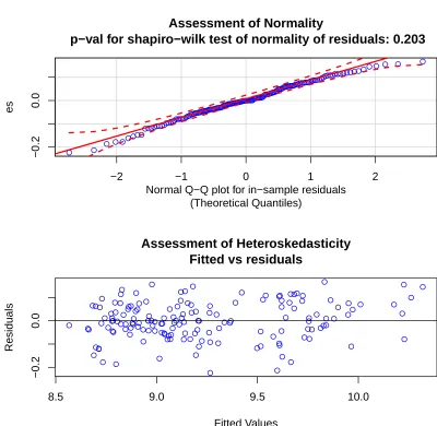
p-val for shapiro-wilk test of normality of residuals: 0.04584
p-val for zero-mean noise: 0.97575
The above output provides a summary for a defaultbartMachinemodel built with
was employed automatically. First, the output prints the dimensions of the design
matrix. Then, it prints the creation time along with other model parameters. Next
the output prints the MSE for the OLS model and displays thebartMachinemodel’s
estimate of σ2
e. We are then given in-sample statistics on error. The pseudo-R2 is
calculated via 1 −SSE/SST. Also provided are outputs from tests of the error
distribution being normal and mean centered . Note that the p-value for
Shapiro-Wilk test of normality of residuals is marginally less than 5%. Thus we conclude
that the noise of Equation 1.8 is not normally distributed. Just as when interpreting
the results from a linear model, non-normality implies we should be circumspect
concerning bartMachineoutput that relies on this distributional assumption such as
the credible and prediction intervals of Section 2.3.4.
We can also obtain out-of-sample statistics to assess level of overfitting by using
k-fold cross-validation. Using 10 randomized folds we find:
R> k_fold_cv(X, y, k_folds = 10)
...
$L1_err
[1] 21.64303
$L2_err
[1] 4.742511
$rmse
[1] 0.1721647
$PseudoRsq
The code provides the out of sample statistics for the model built above. This
function also returns the ˆy predictions as well as the vector of the fold indices (which are omitted in the output shown above).
The Pseudo-R2 being lower out-of-sample (above) versus in-sample suggests that
bartMachine is slightly overfitting (note also that the training sample during
cross-validation is 10% smaller).
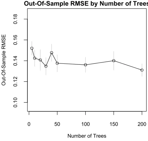
It may also be of interest to see how the number of trees m affects performance.
One can examine how out-of-sample predictions vary by the number of trees via
R> rmse_by_num_trees(bart_machine, num_replicates = 20)
and the output is shown in Figure 2.2. This illustration suggests that predictive
performance levels off around m = 50. We observe similar illustrations across a
wide variety of datasets and hyperparameter choices which is the reason we have set
m= 50 as the default value in the package.
0 50 100 150 200
0.10
0.12
0.14
0.16
0.18
Out-Of-Sample RMSE by Number of Trees
Number of Trees
O
ut
-O
f-Sa
mp
le
R
MSE