http://www.sciencepublishinggroup.com/j/ajam doi: 10.11648/j.ajam.20180602.18
ISSN: 2330-0043 (Print); ISSN: 2330-006X (Online)
Practice of Data Mining in Formative Evaluation
Lintong Zhang, Na Li, Zhigang Zhang
College of Mathematics and Physics, University of Science and Technology Beijing, Beijing, China
Email address:
To cite this article:
Lintong Zhang, Na Li, Zhigang Zhang. Practice of Data Mining in Formative Evaluation. American Journal of Applied Mathematics. Vol. 6, No. 2, 2018, pp. 78-86. doi: 10.11648/j.ajam.20180602.18
Received: May 10, 2018; Accepted: May 18, 2018; Published: June 26, 2018
Abstract:
The main purpose of this paper is to use the students' English learning situation on the Internet to formally evaluate the students' final English performance level. First of all, we introduce the concept of formative evaluation, and the principles of three kinds of data mining algorithms: naive Bayes classification, C4.5 decision tree, and Logistic regression; then, we use the student online learning data table to achieve the key calculation process of the above algorithm; Further, we use Matlab programming to predict the student's final grade level and compare the performance of each algorithm. Practice shows that, C4.5 performs better than Naive Bayes algorithm on predicting the four classifications of grades (great/good/medium/bad), but the accuracy is not very high; Naive Bayes performs better than the other two algorithms and has higher accuracy on predicting the two classifications of grades (good/bad). Considering the two factors of duration of online learning and number of submissions, the accuracy of the prediction has not been significantly improved. Therefore, there is no need to consider both in terms of this formative assessment. Formative assessment has a very important significance in teaching, and plays a key role in motivating students' learning and teacher guidance. According to the forecast results, it can provide some help and guidance for students' follow-up study, so as to improve students' learning effect.Keywords:
Data Mining, Formative Evaluation, Algorithm Performance1. Introduction
Formal assessment is an evaluation of students' learning motivation, learning attitude, learning process and learning effectiveness. The basic idea foundation is to reflect students' learning situation through the students' staged learning process, so as to more objectively evaluate students' achievements in this process.
At present, data mining has been successfully applied in the fields of enterprise management, marketing, and medical care. It is a process of selecting, exploring, and modeling large amounts of data to discover previously unknown rules and relationships. The purpose of data mining is to obtain clear and useful results. As technology matures, data mining is also drawing attention in the field of education, so as to study and solve related problems [1].
This article introduces the concept of formative evaluation and applies this concept to practice. We apply the data mining algorithm to predict the grades of the students' final English grades through the college students' online learning process and compare the performance of the algorithms.
2. The Definition of Formative
Assessment
Formal assessment refers to the evaluation of students' learning situation in the teaching process and the timely detection of problems in teaching and learning. It is often conducted in the form of informal examinations or unit tests.
In this article, we collect the student's English learning on the iSmart software. In the software background, each student submits a record once a time. In the data preprocessing, we integrate the information, submitted by the database, into unit performance data, according to the corresponding weights, so as to predict the final grades through the staged unit grades.
3. The Practice of Formative Assessment
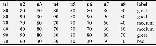
<70)/bad (<60)), and the following data were obtained:
Table 1. Student Online Learning Data Sheet (Four categories).
u1 u2 u3 u4 u5 u6 u7 u8 label
80 80 80 80 80 80 80 90 great 80 90 90 90 80 90 90 80 good 70 70 80 70 70 70 60 40 medium 80 80 80 70 70 70 60 80 medium 90 90 80 80 80 80 80 70 great 70 60 30 30 30 30 30 30 bad
There are 2798 samples of valid data for students who participate in online learning. The following will use three classification methods to predict the students' final test scores, namely: Naive Bayes classification, C4.5 decision tree
classification and Logistic regression classification.
According to the literature review, in the data validation, using Naive Bayes classification, the accuracy is usually low, while the latter two classification methods are highly recommended.
3.1. Naive Bayes Classification
In statistics, Bayes' theorem is used to describe the relationship between two conditional probabilities:
1 1 2 2
1 1 2 2
1 1 2 2
( | , , , )
( ) ( , , , | )
=
( , , , )
n n n n n n
P Y y X x X x X x
P Y y P X x X x X x Y y P X x X x X x
= = = … =
= = = … = =
= = … =
(1)
Y is the decision classes, y is the decision values;xi is
the attribute values in the ith attribute Xi of the sample X
(i=1, 2,…, )n
.
Where P Y( =y) is the class "priori" probability; P X( 1=x X1, 2=x2,…,Xn =x Yn| = y) is the conditional probability of class X relative to the class labelY;1 1 2 2
( , , , n n)
P X =x X =x … X =x is the "evidence" factor used
for the normalization, i.e., the same attribute value of the same attribute of the sample X can be attributed as a class.
Therefore, the problem of evaluating
1 1 2 2
( | , , , n n)
P Y =y X =x X =x … X =x is transformed into
estimating the prior probability P Y( =y) and the class conditional probability P X( 1=x X1, 2= …x2, ,Xn=x Yn| =y)
based on the training sample X .
According to formula (1), the difficulty in finding the posterior probability P Y( =y X| 1=x X1, 2= …x2, ,Xn=xn)
lies in: the class conditional probability
1 1 2 2
( , , , n n| )
P X =x X =x … X =x Y =y is the joint probability
on all attributes, and it is not easy to find directly. In the naive Bayesian classification algorithm, we make an “attribute condition independence Assume" that each attribute is independent of each other [2, 3].
1 1 2 2
1 1 1
( | , , , )
( )
= ( | )
( , , )
n n n
i i i
n n
P Y y X x X x X x
P Y y
P X x Y y
P X x X x =
= = = … =
= = =
= … =
∏
(2)
Y is the decision classes,y is the decision values; xi is
the attribute values in the ith attributeXi of the sampleX
(i=1, 2,…, )n
.
Therefore, the naive Bayes has an expression of:
1 1
1
( , , )
arg max ( ) ( | )
nb n n
n
i i i
h X x X x
P Y y P X x Y y
=
= … =
= =
∏
= = (3)For the attribute value is continuous type, the naive Bayes classification method is to discretize each continuous type of attribute, and then replace the continuous attribute value with the corresponding discrete interval. The data in Table 1 has been processed accordingly. For example, the score in
[
70, 75 is treated as 70, the score between)
[
75,80 is)
treated as 80, and so on.For this algorithm, a 10-fold cross-validation evaluation method is used. Therefore, the training set is 2518 samples and the test set is 280 samples. There are 4 types of tag categories in the student online learning data.
For the data in Table 1, consider the following example to find the corresponding conditional probability:
1470
( )
2518
P label=great =
923
( )
2518
P label=good =
1 70|
41
( 1 70 )
1470
Unit great
P = =P Unit = label=great =
1 70|
120
( 1 70 )
923
Unit good
P = =P Unit = label=good =
2 80|
233
( 2 80 )
1470
Unit great
P = =P Unit = label=great =
2 80|
410
( 2 80 )
923
Unit good
P = =P Unit = label=good =
1 70| 2 80|
( ) Unit great Unit great 0.0026
P label=great ×P = ×P = =
1 70| 2 80|
( ) Unit good Unit good 0.0212
P label=good ×P = ×P = =
Based on the above calculations, it can be concluded that students with a Unit 1 score of 70 and a Unit 2 score of 80 have a higher probability of predicting ‘good’. Therefore, the Naive Bayes classification classifies students in the above situation into ‘good’.
In the following, Naive Bayes classification will be implemented through Matlab programming. We will use 10-fold cross validation to predict the test data, and obtain the confusion matrix and accuracy. Weka software will be used to further obtain the detailed evaluation index under each classification.
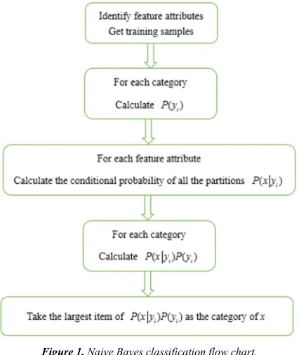
Figure 1. Naive Bayes classification flow chart.
The pseudo code is as follows [4]:
1. Calculate the conditional probability of each independent feature in each category
2. Calculate the probability of occurrence of each category 3. For a specific feature input:
Calculate the conditional probability that it belongs to a specific classification;
4. Select the category with the most probable condition as the input category
Therefore, the naive Bayes has an expression of:
279 632 32 50
162 1437 5 6
56 96 7 13
11 81 1 3
good great medium bad
Taking the "great" level as an example, the classification result classifies 162 students in the great grade of the test set as "good", and classifies the 5 students in the great grade of the test set as "medium"; the 6 tests concentrate on the great grade. Students, judged as "bad"; there are 1437 samples in ‘great’ level correct.
The accuracy calculated by Matlab is 58.5%, but the accuracy is not ideal.
Further, detailed model evaluation indicators are obtained through Weka software:
Table 2. Weka Evaluation Results.
FPR Precision Recall AUC Class
0.127 0.549 0.281 0.548 good 0.620 0.661 0.893 0.853 great 0.014 0.156 0.041 0.725 medium 0.025 0.042 0.130 0.752 bad 0.403 0.585 0.617 0.814
False Positive Rate: The number of negative sample that are predicted to be positive / the number of negative samples
FPR = FP / (FP + TN)
Precision: The number of correct information extracted/the number of extracted information
Recall: the number of correct information extracted/the number of information in the sample
ROC Area (AUC): Area enclosed by FPR-TPR curves When both positive and negative sample sizes are large enough, the ROC curve is sufficient to reflect the model's judgment ability. The value of AUC is the size of the area under the ROC curve. Typically, the AUC value is between 0.5 and 1.0. The larger AUC represents that the algorithm has a better performance. The AUC is a good indicator to evaluate the model. According to the results in the above table, in the ‘AUC’ column, the largest value is the “great” of 0.853. At the same time, the highest accuracy of this level is 0.661, and the recall is 0.893. Therefore, the best rating for classification is “great”.
3.2. C4.5 Decision Tree
In the process of constructing the decision tree, for each node, the C4.5 algorithm selects the attribute with the highest “information gain ratio” as the current splitting attribute, and then continues to calculate the attribute with the highest “information gain ratio” in the left subset as the next node. The C4.5 algorithm uses the “information gain ratio” to select the current node's splitting attribute, which effectively eliminates the disadvantages of “information gain” tending to select the multi-valued attribute [5]. The specific flow chart is as follows:
Figure 2. C4.5 decision tree classification flow chart.
The process of calculating the “information gain ratio” of an attribute is divided into five steps:
1. Calculate category information entropy
represents the probability of each category.
( )
2 1log
m
i i
i
Info D p p
=
= −
∑
(4)2. Calculate the information entropy of each attribute
Assume that the tuples in D are divided according to
attributeA, and attribute A divides D into v different classes. 1 ( ) ( ) v j A j j D
Info D Info D
D =
=
∑
× (5)3. Calculate attribute classification metrics
2 1
( ) log
v j j A j D D splitInfo D D D =
= −
∑
× (6)4. Calculate the information gain
( )
( )
( ) A
Gain A =Info D −Info D (7)
5. Calculate the information gain ratio
( ) ( ) ( ) Gain A GainRatio A SplitInfo A
= (8)
Post pruning - PEP pruning method [6]
If a sub-tree (with multiple leaf nodes) is replaced by a leaf node, the false positive rate on the training set must rise. However, for the test set, the modified decision tree may have a good performance. To eliminate the adverse effects of overfitting when calculating the error rate, we need to add a penalty factor to the miscalculation of the subtree. In the PEP pruning method, the penalty factor is 0.5, and the
miscalculation rate e1 before pruning is calculated as
follows: 1 0.5 i i E L e N + =
∑
∑
(9)i
N =
∑
N represents the number of training samplescovered by this sub-tree,
∑
Ei represents the number of classification errors of the sub-tree, and L represents that the sub-tree has L leaf nodes.The mean number of subtree misjudgments:
( _ ) =e N1 (10)
The standard deviation of sub-tree misjudgment:
( _ ) = e1(1−e N1) (11)
In this case, although a subtree has multiple sub nodes, the subtree miscalculation rate may not necessarily decrease due to the penalty factor.
After the pruning, the internal node becomes a leaf node.
The number of misjudgments J also needs to add a penalty
factor to become J +0.5. The false positive rate e1 after
pruning is calculated as follows:
1 0.5 J e N +
= (12)
The mean number of leaf misjudgments:
( _ ) =e N2 (13)
Pruning standard:
( _ )<( _ )+ ( _ ) (14)
If the pruning criterion is met, that is, the false positive rate after pruning is small, pruning is performed, otherwise pruning is not performed.
For the data in Table 1, the following example illustrates how to calculate the “information gain ratio” in the Unit 1 attribute:
Because it uses a 10-fold cross-validation model assessment method, the training set is 2518 samples and the test set is 280 samples. There are 4 types of tag categories in the student online learning data.
(
)
2 2 1
2
1540 1540 23 23
log log
2518 251
log
( )
0.434 0.529 0.187 0.062
8 2518 25
1.212 18
m
i i
i
Info label p p
= = − = − = + + + = + +
∑
⋯ 1 2 1 2 2( ) log
1 1 5 5
log log
2518 2518 2518 2518
0.004 0.018 1.392
v j j Unit j D D splitInfo D D D = = − × = + + = + + =
∑
⋯ ⋯ 1 12 2 2 2
1
( ) (Unit 1)
1445 1 1 5 5 22 3 3 6 6
log log log log
2518 1445 1445 1445 1445 2518 22 22 22 22
0.574 0.798 0.009 1.693 1.199
v Unit
j Unit
Info label Info
(
)
1(Unit 1)
(Unit 1) 1.212 1.199
1.392 0.0
)
09
(
Unit
Info label Info label GainRatio
SplitInfo
− =
− = =
Therefore, the information gain rate of the attribute Unit 1 is 0.009, according to which the information gain rate of the remaining attributes can be obtained. The attribute corresponding to the maximum value of the information gain ratio is the first node of the decision tree model. The process of constructing a decision tree is recursively implemented according to the above method, and non-leaf nodes of each level are obtained layer by layer.
In the following, the C4.5 decision tree classification algorithm will be implemented through Matlab programming, and a 10 fold cross validation method will be used to predict the test set classification. We will get the confusion matrix and precision, as well as the decision tree model. At the same time, detailed model evaluation indicators are obtained through Weka software.
The pseudo code is as follows [7]: Function TreeGenerate (D, A) 1. Generate node “node”;
2. Select the optimal division attribute a* from A;
3. For each value of a* (indicate by * v
a ): Generate a branch for node;
Let Dv denote a subset of samples in D that have a value
of *
v
a ina*;
Take TreeGenerate (Dv, A\ { }a* ) as the branch node;
4. Return a Decision Tree with “Node” as Its Root Node Get the decision tree as follows:
Unit 1 <= 80
| Unit 8 <= 60: good (125.0/38.0) | Unit 8 > 60
| | Unit 6 <= 70 | | | Unit 7 <= 60
| | | | Unit 2 <= 70: good (20.0/8.0) | | | | Unit 2 > 70
| | | | | Unit 4 <= 70: medium (2.0) | | | | | Unit 4 > 70: great (3.0/1.0) | | | Unit 7 > 60
| | | | Unit 6 <= 60
| | | | | Unit 2 <= 70: good (14.0/7.0) | | | | | Unit 2 > 70: great (4.0/1.0) | | | | Unit 6 > 60
| | | | | Unit 8 <= 70
| | | | | | Unit 1 <= 70: good (29.0/7.0) | | | | | | Unit 1 > 70
| | | | | | | Unit 3 <= 70: great (13.0/5.0) | | | | | | | Unit 3 > 70: good (22.0/8.0) | | | | | Unit 8 > 70: great (53.0/25.0) | | Unit 6 > 70
| | | Unit 5 <= 70
| | | | Unit 8 <= 70
| | | | | Unit 7 <= 70: medium (4.0/1.0) | | | | | Unit 7 > 70: great (2.0)
| | | | Unit 8 > 70 | | | | | Unit 4 <= 70
| | | | | | Unit 6 <= 80: good (10.0/2.0) | | | | | | Unit 6 > 80: medium (4.0/1.0) | | | | | Unit 4 > 70
| | | | | | Unit 7 <= 70: great (4.0/1.0) | | | | | | Unit 7 > 70: good (12.0/1.0) | | | Unit 5 > 70: good (706.0/273.0) Unit 1 > 80
| Unit 4 <= 80: good (320.0/130.0) | Unit 4 > 80
| | Unit 2 <= 80 | | | Unit 6 <= 80
| | | | Unit 3 <= 70: good (2.0) | | | | Unit 3 > 70
| | | | | Unit 5 <= 80: great (9.0/2.0) | | | | | Unit 5 > 80
| | | | | | Unit 3 <= 80: good (6.0/1.0) | | | | | | Unit 3 > 80: great (6.0/2.0) | | | Unit 6 > 80: good (113.0/44.0) | | Unit 2 > 80
| | | Unit 8 <= 80 | | | | Unit 8 <= 60
| | | | | Unit 6 <= 80: good (5.0) | | | | | Unit 6 > 80: medium (2.0/1.0) | | | | Unit 8 > 60
| | | | | Unit 6 <= 80
| | | | | | Unit 5 <= 80: good (11.0/4.0) | | | | | | Unit 5 > 80
| | | | | | | Unit 7 <= 80: great (7.0/1.0) | | | | | | | Unit 7 > 80
| | | | | | | | Unit 3 <= 80: good (2.0) | | | | | | | | Unit 3 > 80: great (6.0/2.0) | | | | | Unit 6 > 80: good (50.0/21.0) | | | Unit 8 > 80
| | | | Unit 3 <= 80: good (51.0/21.0) | | | | Unit 3 > 80
| | | | | Unit 5 <= 80: good (26.0/13.0) | | | | | Unit 5 > 80: great (1155.0/17.0) Get the confusion matrix:
931 61 1 0
437 1173 0 0
163 9 0 0
22 1 0 0
good great medium bad
Table 3. Weka Evaluation Results.
FPR Precision Recall AUC Class
0.345 0.599 0.938 0.802 good 0.060 0.943 0.893 0.852 great 0.000 0.000 0.000 0.711 medium 0.000 0.000 0.000 0.518 bad 0.157 0.599 0.752 0.823
As can be seen from the above table, the classification accuracy of the "great" is as high as 0.943, which is much higher than other levels. At the same time, the AUC value of this level is also the largest. Therefore, the "great" level has the best classification effect.
By comparing the accuracy and AUC values of the above two classification algorithms, the following table can be obtained:
Table 4. Algorithm Performance Comparison.
Naive Bayes C4.5 decision tree
Precision 0.585 0.599
Recall 0.617 0.752
AUC 0.814 0.8230
From Table 4, we can see from the accuracy and AUC, in this topic, the C4.5 decision tree algorithm is better than the naive Bayes algorithm, but the accuracy of the two predictions are not very satisfactory. From a subjective point of view, it may be related to the tag classification method, and may also be related to the classification of the attributes. Therefore, the improvement method is given to improve the prediction accuracy.
3.3. Improvement and Optimization
Divide the tags of student data into good (pass the exam) and bad (fail the exam), so as to convert the above problem into a two-category problem. Here, another two-category algorithm—— the Logistic algorithm, is introduced, this algorithm will be compared with Bayesian classification and C4.5 decision tree classification; further, add two attributes related to online learning in the attribute, namely “learning duration” and “number of submissions”, so as to observe and analyze whether it can improve the prediction accuracy.
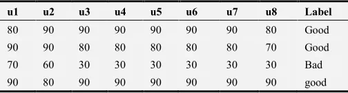
The student data table of two-category problem is as follows:
Table 5. Student Online Learning Data Sheet (Two categories).
u1 u2 u3 u4 u5 u6 u7 u8 Label
80 90 90 90 90 90 90 80 Good 90 90 80 80 80 80 80 70 Good 70 60 30 30 30 30 30 30 Bad 90 80 90 90 90 90 90 90 good
Using the 10-fold cross-validation in the same manner as above, the evaluation index corresponding to the prediction
results of the Naive Bayes algorithm and the C4.5 decision tree algorithm can be obtained.
Confusion matrix of naive Bayes: 2629 130
8 31
good bad
Confusion matrix of C4.5 decision tree: 2754 5
21 18
good bad
The prediction accuracy of the Naive Bayes algorithm is 98.6%, and that of the C4.5 decision tree algorithm is 99.0%.
The C4.5 decision tree is as follows: Unit 1 <= 60
| Unit 4 <= 50
| | Unit 2 <= 60: bad (24.0/1.0) | | Unit 2 > 60: good (3.0) | Unit 4 > 50
| | Unit 5 <= 50: bad (3.0) | | Unit 5 > 50: good (39.0/1.0) Unit 1 > 60: good (2729.0/12.0)
Detailed model evaluation indicators are obtained through Weka software.
Table 6. Weka Evaluation Results in Naive Bayes.
FPR Precision Recall AUC Class
0.205 0.997 0.953 0.376 good 0.047 0.193 0.795 0.376 bad 0.203 0.986 0.951 0.376
Table 7. Weka Evaluation Results in C4.5 Decision Tree.
FPR Precision Recall AUC Class
0.538 0.992 0.998 0.597 good 0.002 0.783 0.462 0.597 bad 0.531 0.990 0.991 0.597
through the Weka software's realization, it is found that the AUC value and recall rate are higher through the Naive Bayes model. Therefore, in the two-category problem of passing the exam, Naive Bayes algorithm has better classification effect.
3.4. Logistic Regression Classification
It is known that ( 1 | ; ) 1 ( )
1 Tx
p y x h x
eθ θ
θ −
= =
+ ≜ ,
1
( 0 | ; ) 1 1 ( )
1 Tx
p y x h x
eθ θ
θ −
= = − −
+ ≜ and Logistic regression
model is:ln 1
T
p x p θ
=
−
. The following is to discuss how to
estimate the parameterθ.
Here, the maximum likelihood estimation method is used to
estimate the parameterθ . According to the steps of the
maximum likelihood estimation method, firstly, the probability function must be obtained:
(
)
1( | ; ) ( ) (1y ( )) y
p y x
θ
= h xθ −h xθ − (15)Because the sample data (m pieces) are independent, their joint distribution can be expressed as the probability of each edge distribution, and the likelihood function is obtained:
(
)
( )( )
( ) ( ) 1
1
( ) ( ) (1 ( ))
i
i
m
y
i i y
i
Lθ h xθ h xθ −
=
=
∏
∗ − (16)Logarithm to the likelihood function:
( ) ( ) ( ) ( )
1
( ) ln( ( )) (1 ) ln(1 ( ))
m
i i i i
i
lθ y h xθ y h xθ =
=
∑
+ − − (17)The maximum likelihood estimation is to solve θ such
that l( )θ obtains the maximum value, so the log likelihood function is derived:
( ) ( ) ( )
1
( ( )) 0
m
i i i
i
l
y h xθ x
θ =
∂ = − ⋅ =
∂
∑
(18)For the above formula, the analytical solution cannot be obtained directly. Here, the gradient analysis algorithm in the optimization method is used to obtain the corresponding analytical equation.
For the gradient descent algorithm, the following is the iteration formula:
( 1) ( )
1
1
( ( ) )
m
n n
i i i i
h x y x m θ
θ + θ α
=
= −
∑
− (19)Through the above iteration, the estimated value of θ can
be obtained, and then the obtainedθ is brought into the Logistic regression model, and the probability that the ith sample is classified into ( )
1
i
y = is:
( )
( )
( ) ( )
( )
1
T i T i
x
i i
x e
p h x
e
θ
θ θ
= =
+ (20)
If ( )
0.5
i
p > , the sample is classified as “1” class, otherwise
it is classified as another class [9].
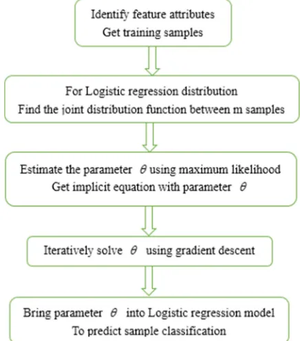
The logistic regression flow chart is as follows:
Figure 3. Logistic regression classification flow chart.
The pseudo code is as follows [10]:
1. Each regression coefficient is initialized to 1 2. Repeat R times:
Calculate the gradient of the entire data set;
Update the regression coefficient vector with
alpha*gradient;
3. Return the regression coefficient
The following will implement the Logistic regression classification algorithm through Matlab programming [11], and use 10 fold cross validation method to predict the test set, and then, we can get the confusion matrix and accuracy, at the same time, we will use Weka software to further obtain
the value of the parameterθ , and the model evaluation
indicators.
Confusion matrix of Logistic: 756 3
18 21
good bad
The accuracy of the algorithm is 99.25% obtained by Matlab, and the accuracy is higher than that predicted by Naive Bayes and C4.5 algorithm.
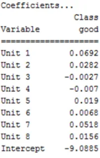
Figure 4. Logistic regression coefficients.
Table 8. Weka Evaluation Results in Logistic Regression.
FPR Precision Recall AUC Class
0.462 0.994 0.999 0.890 good 0.001 0.875 0.538 0.890 bad 0.455 0.992 0.992 0.890
Using naive Bayes, C4.5 decision tree and Logistic regression algorithm to predict the final score of the passing situation, the following prediction results are obtained:
Table 9. Algorithm Performance Comparison.
Precision Recall FPR AUC
Bayes 0.99 0.99 0.21 0.91 C4.5 0.99 0.99 0.54 0.78 Logistic 0.99 0.99 0.46 0.89
Through the analysis of the above table, in the problem of predicting “passing the exam”, the Naive Bayes classification algorithm shows a good prediction performance, with the highest AUC value, and the false positive rate is much lower than the other two algorithms. Therefore, the Naive Bayesian classification algorithm can be used to predict the students' English exam passing.
3.5. Exploration and Discovery
Considering that duration of learning and the number of submissions for students' online learning are also related to the final grades of English, therefore, on the basis of the above, two attributes are added to predict the “pass/fail”. The following data sheet is obtained:
Table 10. Student Online Learning Data Sheet (Concluding duration of learning and the number of submissions).
u1 u2 u3 u4 u5 u6 u7 u8 seconds count label
90 90 80 80 80 80 80 70 30520 795 Good 70 60 30 30 30 30 30 30 6083 328 Bad 90 80 90 90 90 90 90 90 22648 391 good 90 90 90 80 90 90 90 80 18065 210 good
Use the above three algorithms to model the data, and
predict “pass/fail”. Here, get the following table:
Table 11. Algorithm Performance Comparison.
Precision Recall FPR AUC
Bayes 0.99 0.99 0.21 0.94 C4.5 0.99 0.99 0.51 0.75 Logistic 0.99 0.99 0.49 0.92
According to the analysis of the results in Table 11, we can see that if we consider duration of learning and the number of submissions, the prediction accuracy and recall rate will not be significantly improved, and the false positive rate of the C4.5 algorithm will decrease slightly. Naive Bayesian The logistic regression algorithm's AUC value will increase slightly. Therefore, in summary, when we formatively assess the effect of students' online learning situation on passing the exam, there is no need to consider duration of learning and the number of submissions [12].
4. Conclusion
This paper studies the formative evaluation and applies two algorithms: Naive Bayes and C4.5 decision tree, to mining data in students' online learning, and uses Matlab programming to predict students' final exam of four classifications (great/good/medium/bad). According to the evaluation results, it is found that the performance of the C4.5 decision tree is superior to the Naive Bayes algorithm in this problem, but the result is not very satisfactory. Next, the data label classification is changed from four categories to two categories, in order to predict students' final exam of two classifications (good/bad), and then we introduce Logistic regression. We use the above three algorithms to perform data mining similarly. From the results, we can see that Naive Bayes performs better than other algorithms under this problem, and has achieved a high degree of accuracy. Further, we use the database to obtain two attributes of students' online learning: duration and number of submissions, and add them to the data table. These three algorithms are also used for mining. According to the evaluation results, the prediction performance is not significantly improved than before. Therefore, it is concluded that there is no need to consider the duration of learning and the number of online submissions when studying the data of this group of formative evaluations. Above all, this paper uses data mining technology to form learner’s formative evaluation of online learning, and then, provides learners with timely and effective evaluation feedback, so as to help learners identify problems in the learning process, continuously improve their own learning, and give full play to the advantages of formative evaluation, so that learners can continuously improve.
Acknowledgements
Science and Technology Education Research Project (JG2017Z10).
References
[1] Ding Bo. Research on subdivision prediction of online learning students' academic achievement [D]. Jiangnan University, 2016.
[2] Cheng Kefei, Zhang Cong. Naive Bayesian Classifier Based on Feature Weighting [J]. Computer Simulation, 2006, 23 (10):92-94.
[3] Mladenic D, Grobelnik M. Feature Selection for Unbalanced Class Distribution and Naive Bayes [C]. Sixteenth International Conference on Machine Learning. Morgan Kaufmann Publishers Inc. 1999:258-267.
[4] Rish I. An empirical study of the naive Bayes classifier [J]. Journal of Universal Computer Science, 2001, 1 (2):127. [5] Quinlan J. R. C4.5: programs for machine learning [M].
Morgan Kaufmann Publishers Inc. 1993.
[6] Quinlan J R. Improved Use of Continuous Attributes in C4.5 [J]. Journal of Artificial Intelligence Research, 1996, 4 (1):77-90.
[7] Wang Xiaoguo, Huang Yukun, Zhu Wei, et al. Application of C4.5 Algorithm to Construct Customer Classification Decision Tree [J]. Computer Engineering, 2003, 29 (14):89-91. [8] Choi In-ho. The application of data mining in student
professional achievement prediction [J]. Software, 2016, (01): 24-27.
[9] Wang Jichuan, Guo Zhigang. Logistic Regression Model: Method and Application [M]. Higher Education Press, 2001. [10] Zheng Yinan, Cao Peihua, Ou Chunquan. Realization of N:M
Conditional Logistic Regression Analysis on Statistical Software [J]. Chinese Journal of Health Statistics, 2011, 28 (1):93-94.
[11] Tan Hongwei, Zeng Jie. Impact Analysis of Logistic Regression Model [J]. Mathematical Statistics and Management, 2013, 32 (3): 476-485.