University of Windsor University of Windsor
Scholarship at UWindsor
Scholarship at UWindsor
Electronic Theses and Dissertations Theses, Dissertations, and Major Papers
12-17-2015
Constrained optimization for bottleneck peak hour pricing
Constrained optimization for bottleneck peak hour pricing
Da Xu
University of Windsor
Follow this and additional works at: https://scholar.uwindsor.ca/etd
Recommended Citation Recommended Citation
Xu, Da, "Constrained optimization for bottleneck peak hour pricing" (2015). Electronic Theses and Dissertations. 5678.
https://scholar.uwindsor.ca/etd/5678
This online database contains the full-text of PhD dissertations and Masters’ theses of University of Windsor students from 1954 forward. These documents are made available for personal study and research purposes only, in accordance with the Canadian Copyright Act and the Creative Commons license—CC BY-NC-ND (Attribution, Non-Commercial, No Derivative Works). Under this license, works must always be attributed to the copyright holder (original author), cannot be used for any commercial purposes, and may not be altered. Any other use would require the permission of the copyright holder. Students may inquire about withdrawing their dissertation and/or thesis from this database. For additional inquiries, please contact the repository administrator via email
CONSTRAINED OPTIMIZATION FOR BOTTLENECK PEAK HOUR PRICING
By
Da Xu
A Thesis
Submitted to the Faculty of Graduate Studies through Mechanical Engineering in Partial Fulfillment
of the Requirements
for the Degree of Master of Applied Science at the University of Windsor
Windsor, Ontario, Canada
2015
CONSTRAINED OPTIMIZATION FOR BOTTLENECK PEAK HOUR PRICING
by
Da Xu
APPROVED BY:
Dr. L. Oriet Mechanical Engineering
Dr. L. Zhong Odette School of Business
Dr. X. Guo, Advisor Odette School of Business
Dr. G. Zhang, Advisor Mechanical Engineering
iii
DECLARATION OF ORIGINALITY
I hereby certify that I am the sole author of this thesis and that no part of this thesis has been
published or submitted for publication.
I certify that, to the best of my knowledge, my thesis does not infringe upon anyone’s copyright
nor violate any proprietary rights and that any ideas, techniques, quotations, or any
other material from the work of other people included in my thesis, published or otherwise,
are fully acknowledged in accordance with the standard referencing practices. Furthermore, to the
extent that I have included copyrighted material that surpasses the bounds of fair dealing within
the meaning of the Canada Copyright Act, I certify that I have obtained a written permission from
the copyright owner(s) to include such material(s) in my thesis and have included copies of such
copyright clearances to my appendix.
I declare that this is a true copy of my thesis, including any final revisions, as approved by my
thesis committee and the Graduate Studies office, and that this thesis has not been submitted
iv
ABSTRACT
We study the morning commute problem with a peak period flat toll, where the toll has a maximum
acceptable toll level and a maximum acceptable length of tolling period. Under such a constrained
optimization setup, we investigate the system cost minimization problem. A tolling scheme is
determined by the toll starting time, the toll ending time, and the toll level. The toll starting time
and ending time are set before and after the common work start time, respectively. We find out
that, under the toll window length constraint only, a balanced toll window design is always optimal,
where “balanced” means that the part of the toll window before the work start time and the part
after have equal monetary value. Under both the toll level and the toll window length constraints,
the balanced design is optimal if feasible; otherwise the toll should start later with the same toll
v
ACKNOWLEDGEMENTS
To grandma, for your everlasting love and bless to me.
To my supervisor, Dr. Xiaolei Guo, for guiding me and inspiring me through the completion of
this thesis. Thank you for spending so much time talking with me for my life. You are always my
respected mentor.
To my supervisor, Dr. Guoqing Zhang, for providing me precious comments to improve this thesis
and helping me obtain this degree. I cherish every time we talk in your office. Those moments
were happy and unforgettable.
To my committee members, Dr. Leo Oriet and Dr. Ligang Zhong, for your insightful ideas and
recommendations to finalize this thesis. Your ideas enlightened me in so many aspects of my
research. Thank you for giving me so much inspiration for my future work.
vi
TABLE OF CONTENTS
DECLARATION OF ORIGINALITY ... iii
ABSTRACT... iv
ACKNOWLEDGEMENTS ... v
LIST OF TABLES ... vii
LIST OF FIGURES ... viii
1. INTRODUCTION ...1
2. LITERATURE REVIEW………. 5
3. EQUILIBRIUM OF UNTOLLED SINGLE BOTTLENECK ... 7
4. EQUILIBRIUM OF TOLLED SINGLE BOTTLENECK………... 9
5. UNCONSTRAINED OPTIMIZATION PROBLEM……….. 23
6. CONSTRAINED OPTIMIZATION PROBLEM……….... 29
6.1 Scenario One... 30
6.2 Scenario Two………. 30
6.3 Scenario Three………... 38
6.4 Scenario Four………. 40
7. NUMERICAL EXAMPLE... 41
8. CONCLUSION ………. 46
REFERENCES……… 47
APPENDIX A……….. 49
APPENDIX B ………..52
APPENDIX C……….. 63
vii
LIST OF TABLES
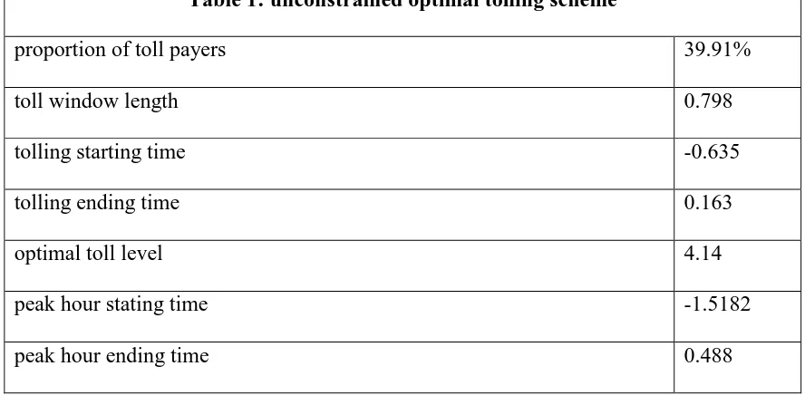
Table 1: unconstrained optimal tolling scheme....………....41
Table 2: constrained optimal tolling scheme with l0.75……….42
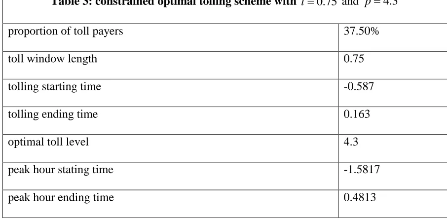
Table 3: constrained optimal tolling scheme with l0.75 and p4.3……….43
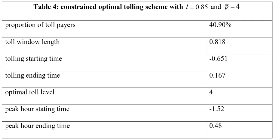
Table 4: constrained optimal tolling scheme with l0.85 and p4………44
Table 5: constrained optimal tolling scheme with l0.75 and p4………44
Table 6: constrained optimal tolling scheme with l0.75and p4.6………..45
viii
LIST OF FIGURES
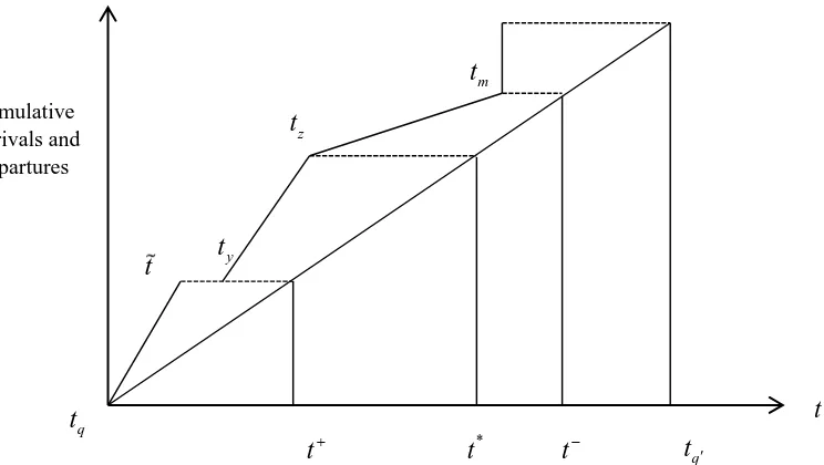
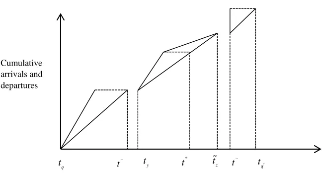
Figure 1: untolled single bottleneck equilibrium profile………8
Figure 2: equilibrium profile of tolled bottleneck without capacity waste………9
Figure 3: complete tolled single bottleneck equilibrium profile………18
Figure 4: equilibrium profile of capacity waste at both t and t……….52
1
1. Introduction
In recent decades, the problems stemming from high vehicle ownership and heavy road usage has
become much starker. These problems include road congestion, pavement damage, air pollution,
traffic accidents and limited parking places. As a result, road pricing has been widely implemented
all over the world. The world's first congestion tolling scheme was introduced in Singapore's core
central business district (CBD) in 1975 as the Singapore Area Licensing Scheme (ALS). The roads
leading to the CBD are tolled. If a driver wants to enter the CBD, she needs to purchase a special
paper license which is sold at post offices, gas stations or convenience stores, on a monthly or
daily basis. The toll gate at the entrance of the CBD are gantries where police officers are visually
checking the license and recording any violations. The ALS was upgraded to 100%
free-flowing Electronic Road Pricing (ERP) system in September 1998. Sensors are installed on the
gantries to communicate with an In-vehicle Unit (IU) to implement the charging. The IU is a device
to insert a cash card to pay the toll. When a car drives under a gantry, the sensors on the gantry
will work with the IU to deduct the money in the cash card automatically. Each registered car
intending to enter the CBD is enforced to install an IU by law. Actually, before Singapore’s
implementation of ERP, Hong Kong experimented the ERP system during 1983 to 1985. The
results demonstrated the technical feasibility of this tolling system, but it was aborted due to the
public opposition. In Europe, Norway implemented a cordon tolling scheme in the city of Bergen
(1986), Oslo (1990) and Trondheim (1991). The Oslo toll ring is a classic cordon pricing scheme
with 19 toll stations circling the centre of Oslo. People driving into the city need to pay a fee when
they pass the cordon line. The toll stations support electronic payment without reducing vehicle’s
2
so the city centre’s traffic congestion can be effectively alleviated. The collected toll is intended
to improve road network and finance road construction projects. Sweden introduced Stockholm
congestion tax that covers Stockholm city centre in August 2007. All the entrances and exits of
the centre area have unmanned control points operating with automatic number plate recognition.
Vehicles entering this are during the peak hours need to pay a fixed fee. The congestion tax
collected from commuters is also used to construct and maintain the toll roads. US first introduced
the High-occupancy toll lane (HOT lane) system in 1995 on California’s 91 express lanes. In next
year, Interstate 15, north of San Diego, also started to implement the HOT tolling scheme. The
HOT lane is a traffic lane that is only free to high-occupancy vehicles and designated exempt
vehicles. The high occupancy vehicle usually is the vehicle with at least 2 or 3 occupants. Other
vehicles intending to use the lane need to pay a toll. If the driver does not like to pay the toll, she
can also use the general untolled lane. The toll level is displayed at the entry of the lanes, which is
adjusted according to the travel demand to control traffic volume to ensure the minimum traffic
speed and service level.
In urban area, during the morning commute peak hours, heavy congestion at road’s bottleneck has
now become an unneglectable problem for the commuters. It is very common to hear one’s
colleague complaining how long she has to wait on the road. Since no one would like to come to
workplace too early or can afford the penalty of being late, travelers usually depart from home at
approximately same time periods. At the road’s bottleneck section, due to its capacity limit to
handle the travel demand, congestion is inevitable. Motivated by this problem, this thesis proposes
a tolling scheme implemented during morning commute peak hours. Our purpose is to alleviate
3
bottleneck area which usually has very limited capacity. We choose to charge a coarse toll because
of its easiness to implement. The dynamic toll or the time-varying toll can cause confusion to the
commuter, as the commuter may not know when she should depart from home. In this thesis, the
bottleneck model is built based on the concept of equilibrium. At equilibrium, no commuter can
further reduce her travel cost by altering the arrival time at the bottleneck. By levying a toll on the
bottleneck, the equilibrium profile of commuters could have a tremendous change compared with
the no-toll scenario. Considering that the toll has a maximum public acceptable level and the tolling
period has a maximum public acceptable length, we investigate the problem of system cost
minimization and our goal is to find the optimal tolling scheme under these two constraints. Under
the optimal tolling scheme, commuters have the minimum total system cost. It could also be
understood as the best equilibrium profile of all profiles. Under such a constrained optimization
setup, we first solve the equilibrium of the bottleneck model. We find out that, for any toll window,
there exists a critical toll level over which capacity waste can happen. Capacity waste is a time
period during which, no commuter uses the bottleneck. Then, based on the individual cost, we
prove, in respect of total system cost, a tolling scheme without capacity waste is always better than
a scheme with capacity waste. We also find out that, under toll window length constraint only, if
the unconstrained optimal tolling scheme is infeasible, we should push toll window length to the
upper bound, make toll window balanced and charge the corresponding critical toll price. Balanced
means the part of the toll window before the work start time and the part after has equal monetary
value. Under both toll level and toll window length constraints, if the unconstrained optimal tolling
scheme is infeasible, whenever possible, a balanced toll window and its corresponding critical toll
price can solve the problem; if the balanced design gives a critical toll price exceeding the upper
4
namely make the toll window unbalanced, and charge the corresponding critical toll price of the
moved toll window.
The remainder of this thesis is organized as follows. In chapter two, we do a literature review to
show the previous researches of the road bottleneck model. In chapter three, we review the
equilibrium of untolled bottleneck model. Chapter four gives a complete picture of tolled
bottleneck model, where we investigated the equilibrium profiles of different tolling schemes. In
chapter five, we solve the unconstrained system cost optimization problem based on the individual
cost. In chapter six, we solve the constrained system cost optimization problem given both toll
level and toll window length constraints. In chapter seven, we use numerical examples to
demonstrate the proposed optimal tolling schemes under different constraint setups. Concluding
remarks are offered in chapter eight.
5
2. Literature Review
To model the morning commute problem, Vickery first introduced the road bottleneck model in
1969 (Vickery 1969). Hendrickson and Kocur (1981) reviewed the no-toll equilibrium of
bottleneck model with and without no lateness assumption. They also investigated the distribution
of work start times and pointed out that the condition of equilibrium is that the arrival rate of
commuters must be constant. As bottleneck model’s pioneers, Arnott et al. (1988) extend
Vickery’s model by assuming different work starting times. They investigated users’ no-toll
equilibrium profile and showed that, for two groups of commuters, the queue at the bottleneck can
be single peaked, double peaked or the rush hour can be separate based on the work starting times’
difference. Arnott et al. (1990) pointed out by levying a flat toll during the commuting period,
travelers’ total system cost can be reduced and under the optimal tolling scheme, there should be
no queue at the toll window’s endpoints. Arnott et al. (1993) extended Vickery’s model further by
assuming elastic demand and found the optimal road capacity under various pricing regimes.
Arnott et al. (1994) examined the welfare effects of the optimal time-varying toll. In their model,
the commuters are divided into several groups, each group with its own unique VOT but shares
same relative cost of late to early arrival. Under the time-varying toll, queue is completely
eliminated but such a tolling scheme depends on each group’s VOT and travel demand. In real
world it is very inconvenient to implement and can also be quite confusing to commuters, besides
their model does not consider continuous VOT distribution either. Further effort was made to
reduce commuters’ queuing delay at the bottleneck, such as Laih (1994) proposed a multi-step
tolling scheme where different flat tolls are levied on different time periods during the peak hour.
6
flat toll does not change commuter’s travel cost (compared with no-toll equilibrium). Although
under the optimal time-varying toll, the toll revenue equals the saved queuing cost, it is usually
not true under a flat toll. Lindsey (2004) reviewed previous bottleneck models under assumption
of multiple user classes and proved the existence and uniqueness of user equilibrium of bottleneck
model. Xiao et al. (2011) extended Arnott’s model (1990) by providing details of how the queuing
profile changes with respect to toll level under heterogeneous VOT assumption. They formulate a
non-linear optimization problem to solve the equilibrium and find out the optimal tolling scheme.
Under their optimal tolling scheme, no queue exists at toll window’s endpoints either. This is
mainly due to the proportional assumption of user’s VOT. Xiao et al. (2013) extend Arnott’s model
(1994) by assuming continuous VOT distribution, where social optimum is also achieved by a
dynamic tolling scheme. Under his model, the toll level only depends on each commuters’ VOT
and does not require dividing travelers into groups, which can save some work but such a dynamic
tolling scheme also suffers from inconvenience of implementing.
Based on our literature review, none of the existing works studied the constrained optimization
problem of a tolled bottleneck. For public acceptable issue, we consider that the toll has a
maximum acceptable toll level and a maximum acceptable length of tolling period, both
exogenously given, so a constrained system optimization problem can be proposed. In this thesis,
we still use flat toll for our tolling scheme as it is easy to be implemented in real world. We will
solve the constrained system cost optimization problem given both toll level and toll window
7
3. Equilibrium of Untolled Single Bottleneck
During the morning commute peak hours, at some busy roads, we can easily observe travelers
stuck by heavy congestion. This is usually due to most commuters have roughly same work starting
time but the capacity of the road cannot satisfy such high travel demand. In order to model this
phenomenon, bottleneck model is introduced. In this section, we will briefly review the
equilibrium of untolled single bottleneck during the morning commute period for users with
heterogeneous VOT. t* is assumed to be commuters’ preferred arrival time at work. If a commuter arrives at work before t*, she will be incurred a schedule early delay cost . If she arrives at work later than t* she will be incurred a schedule late delay cost . The queuing delay cost is denoted by . We assume and , where and are constants
0 1
. The xth user’s VOT
x is assumed to be a monotonically decreasing function with respect to x. The total number of commuters is assumed to be N . The bottleneck’s capacityis s. The arrival rate is denoted by . When commuter’s arrival rate is higher than s, a queue will develop at the bottleneck. When commuter’s arrival rate is lower than s, the queue at the bottleneck will gradually dissipate. Since and are both constants, the profile of the no-toll
equilibrium should be pretty similar with the equilibrium profile under homogeneous VOT
assumption. At equilibrium, the arrival rates of commuters having schedule early and late delay
can be obtained as both constants, implying the traveler’s position in the queue is random. Since
we assume commuters value schedule late delay more than schedule early delay, we can see in
figure 1 the arrival rate of commuters having schedule early delay is much higher than that of
8
We can obtain t* tq N
s and tq t* N
s. Figure 1 shows the untolledsingle bottleneck equilibrium profile of users having heterogeneous VOT. (See Appendix A for
details)
9
4. Equilibrium of Tolled Single Bottleneck
In this section we will talk about the equilibrium of tolled single bottleneck with commuters having
heterogeneous VOT. A flat toll p is imposed from t to t. Our tolling scheme only assumes *
t t t. At equilibrium no traveler can further reduce her travel cost by adjusting her arrival time at the bottleneck. Since the flat toll has no impact on toll payers’ travel time choice, the arrival
pattern of toll payers having schedule early delay or late delay should be similar with those under
the profile of untolled single bottleneck. As the toll non-payer who arrives before t is incurred a schedule early delay cost, her arrival rate should be similar with that of the toll payer who also has
schedule early delay cost. The arrival rate of travelers having schedule early delay can be obtained
as s1. The arrival rate of travelers having schedule late delay can be obtained as s 1.
q
t
t
t t
y
t
z
t
*
t
m
t
q
t
cumulative arrivals and departures
t
10
When the toll window length is not too long and toll level is not too high, the bottleneck can be
fully utilized with no capacity waste. Here capacity waste means a period during which no queue
exists at the bottleneck between the arrival time of the first and last commuter. The xth commuter is assumed to be the toll non-payer arriving before t, her travel cost can be given by
1
1
*
, q q
t t
q q
t d s t t t d s t t
C x t x x t t
s s
At equilibrium, we can obtain
*
, q
C x t x t t (1)
As the bottleneck is fully utilized, the first toll payer should come no later than t. The yth commuter is assumed to be the toll payer who experiences schedule early delay, her cost can be
given by
1 2
1 2
*
, q y
q y
t t
q
t t
t t
q
t t
d d s t t
C y t y
s
d d s t t
y t t p
s
where t is the arrival time of the last toll non-payer arriving before t. ty is the arrival time of first toll payer. At equilibrium, we can obtain
*
, y
C y t y tt y t t p (2)
11
1 2 3
1 2 3
* ,
z
q y z
z
q y z
t t t
q
t t t
t t t
q
t t t
d d d s t t
C z t z
s
d d d s t t
z t t p
s
where traveler who arrives at tz experiences no schedule early or late delay, since she is cleared just at t*. At equilibrium, we can obtain
*
, z
C z t z t t p
Mass arrival happens right after the arrival time of the last toll payer. We denote it by tm. Every
commuter in the mass arrival is assumed to experience an average queuing delay and schedule late
delay of the total mass. The travel cost of commuter in the mass arrival can be given by
*,
2 2
q q
m m
t t t t
C m t m t m t
At equilibrium, the indifferent user is the commuter who can arrive at any time as she is always
incurred identical travel cost. For those who have higher VOT than the indifferent user, they will
pay the toll to pass the bottleneck. For those who have lower VOT than the indifferent user, they
will avoid the toll by coming earlier or later. The toll price can be easily obtained as the queuing
cost difference of the indifferent user arriving at t and ty respectively, thus we have
y
ps tt t t
From
1 q q
s
t t s t t
*
1 z y
s
t t s t t
12
*
1 m z
s
t t s t t
q q N t t s
we can further obtain
2 1 q p N t t s s t t (3)
1
2 1 1 2 2 y q N t s
t t t
*
2 1 1 2 2 m q N t st t t
From (3), we can see when toll price is increased, the first commuter will postpone her arrival.
Since the first commuter has postponed her arrival, the first and last toll payer will also postpone
their arrivals or we can say the equilibrium profile will move rightward. When toll price is
increased to a certain level, the first toll payer will arrive exactly at t or the last toll payer will arrive exactly at t. At this moment, if we keep increasing the toll level, capacity waste will occur at tort. By setting ty t
, we can obtain
1
1
2 1
s t t N
p t t
s
(4)
If toll window is designed as
*
*
t t t t
, t t N s and toll level is kept within
1
0 p p , the bottleneck will be fully utilized. This corresponds to area AODin figure 2. By
13
*
2
1
2 1
N
p s t t t t
s
(5)
If toll window is designed as
t*t
tt*
, t t* N
s and toll level is keptwithin 0 p p2, the bottleneck will be fully utilized. This corresponds to area ODFin figure 2.
If toll window is designed balanced as
*
*
t t t t
, we have
1 2
p p . If toll level is
pushed to p1 or p2, the first and last toll payer will arrive exactly at t and t, which implies no queue exists at the endpoints of the toll window. This corresponds to line OD in figure 2.
When toll level exceeds p1 or p2, depending on the design of toll window, capacity waste will start to occur at t, tor even at both tand t. If the toll window satisfies
*
*
t t t t
,
when toll level is pushed above p1, capacity waste will only occur at t. Using the same logic, if the toll window is designed as
t*t
tt*
, when toll level exceeds p2, we will observecapacity waste only at t. Of course, for the design of
t*t
tt*
, when toll price surpasses p1 or p2, capacity waste will occur at both t and t.If capacity waste only exists at t, during
t t, y
no queue exists at the bottleneck. From the standpoint of the indifferent user we can easily obtain the toll price as the travel cost difference ofher coming as the first toll non-payer and first toll payer respectively, thus we have
y q
14
where is the proportion of toll payers. The Nth commuter is namely the indifferent user. She has the lowest VOT among the toll payers but the highest VOT among the toll non-payers. The
toll price is simply the schedule early delay difference of her coming at these two moments. Based
on the fundamental equilibrium relations, we can obtain
*
m
N
t t t t
s
12
1 2
N N
p N t t
s s
where
y
N
t t s
It is shown the toll price is a function of toll payers’ proportion. When toll level is raised up, the
indifferent user’s VOT will increase. As fewer people can afford the toll, toll payers can gain more
time choice freedom. The last toll payer is going to postpone her arrival by arriving closer to t. When toll price is raised to a certain level, the last toll payer will arrive exactly at t. By setting
m
t t, we have
*
*
*
3
1
2
1 2
N
p s t t t t t t
s
(6)
If the toll window is designed as
t*t
tt*
, t t N s and toll price is kept within1 3
15
When toll level exceeds p3, capacity waste will also occur at t. If we have capacity waste at t, since there is no queue, the mass arrival should happen exactly at t. If we denote tz as the last toll payer’s arrival time, from the standpoint of the indifferent user, we should have
*
*
y z
t t t t
This implies the first toll payer’s schedule early delay equals the last toll payer’s schedule late
delay. The toll price can be obtained as
2
*
1 2 2 2 2 2 3
1 2 1 1
z y z
N
p s t t t t t t
s
where s t
z ty
is the indifferent user’s VOT.It is easy to understand when toll price is pushed high enough, only the zeroth person (commuter
with highest VOT) can afford the toll to pass the bottleneck. The rest commuters have to come
either before t, or after t. It is obvious the zeroth commuter should arrive exactly at t*, since she will not be incurred any schedule delay cost. Such a toll price can be obtained by setting tz t*. By setting tz t*, we can obtain
*4
1 2 1
0
1 2 1 1
N
p t t t
s
(7)
By setting tz t, we can obtain
*
1
*
*
2
1 2
N
p s t t t t t t
s
If the toll window is designed as
t*t
tt*
, t t N s and toll level is kept within3 4
16
When toll price is greater than p4, no commuter can afford the toll, all of them arrive either before
t or join the mass arrival at t. (Figure 2 area AOD)
Now let us talk about capacity waste only existing at t. If the toll window design satisfies
*
*
t t t t
, when toll level exceeds p2, capacity waste will only occur at t. Since there is no queue between tz and t, mass arrival will happen exactly at t. The toll price can be obtained as the indifferent user’s travel cost difference of her coming at tq and ty respectively, thus we have
q
y
p N tt N tt
The toll price can be understood as the travel cost difference of indifferent user arriving as the first
toll non-payer and first toll payer respectively. Based on the fundamental equilibrium relations,
we can obtain
*
*
y z
t t t t t t
2
* 1 3 21
2 1 2 2 2
N N
p N t t t
s s
where
z
N
t t s
We can see the toll price is a function of toll payers’ proportion. When toll price is increased, the
indifferent user’s VOT will correspondingly increase. As fewer people can afford the toll, the toll
17
closer to t. Finally when toll price is increased to a certain level, the first toll payer will arrive exactly at t and at this moment if we keep raising the toll level, capacity waste will also occur at
t. By setting ty t
, we could obtain
2
2
2
* * *
5
2 3
2 1 2 1 2 1
N
p s t t t t t t
s
(8)
If toll window is designed as
t*t
tt*
, t t* N
s and toll level is keptwithin p2 p p5, capacity waste only occurs at t. This corresponds to area ODFin figure 2.
When toll level exceedsp5, capacity waste will also occur at t. Using the same logic, we can see if toll level is kept within p5 p p4, capacity waste occurs at both t and t. (Figure 2 area
ODF)
When toll price is higher than p4, no commuters will use the toll window. All of them will arrive
either before t or after t. (Figure 2 area ODF)
For the balanced toll window design, we have p1 p2 p3 p5, so when toll level exceedsp1 but
18
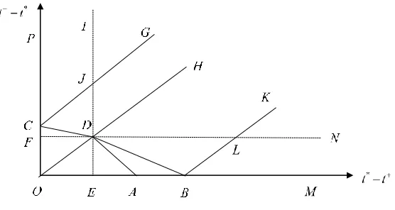
Figure 3: complete tolled single bottleneck equilibrium profile
The following equations are the lines in figure 3.
*
*
:
OH t t tt ,
*
*
: N
CG t t t t
s
, D: N, N
s s
*
*
1:
2 N
BK t t t t
s
,
*
*
: N
AD t t t t s
2 * *: 2 1 N
BD t t t t
s
, CD:
t* t
t t*
N s
The equilibrium profile is not only restricted to what we have discussed above. In the following,
we will give a full picture of commuter’s equilibrium patterns. (See Appendix B for details) We
let
6
1 2 1
1 2 1 2 1 2
N s N
p t t t t
s
*
*
7 Np s t t t t
19
*
*
*
*8
2 N
p s t t s t t N t t t t
s
*
9 Np N t t
s
* 10 0 Np t t
s
2
* * * *
11
N
p s t t s t t N t t t t
s
*
*
12 1 2 Np s t t t t
s
* * 13 2 2 * * 2 2 1 11 2 2
1 1
s s
p N t t t t
N
t t t t
s
*
14 1 0 2 Np t t
s
*
15 Np N t t
s
In area ADB: when 0 p p6, no commuter arrives before t, no capacity waste occurs at t, mass arrival occurs before or at t; when p6 p p3, commuter arrives before t, capacity waste only occurs at t, mass arrival occurs before or at t; when p3 p p4, commuter arrives before
20
In area CDJ : when 0 p p7, bottleneck can be fully utilized but has no mass arrival; when
7 8
p p p , capacity waste only occurs at t and there is no mass arrival; whenp8 p p4, mass arrival recurs at t, capacity waste occurs at both t and t.
In area GJDH : when p9 p p8, capacity waste only occurs at t and there is no mass arrival; when p8 p p4, mass arrival recurs at t, capacity waste occurs at both t and t.
In area PCJI: when 0 p p7, bottleneck can be fully utilized but has no mass arrival; when
7 10
p p p , capacity waste only occurs at t and there is no mass arrival.
In area IJG: when p9 p p10, capacity waste only occurs at t and there is no mass arrival.
In area CFD: when 0 p p11, bottleneck can be fully utilized but has no mass arrival; when
11 5
p p p , capacity waste only occurs at t and mass arrival occurs at t; when p5 p p4, capacity waste occurs at both t and t, mass arrival occurs at t.
21
In area NLBM : when 0 p p12, no commuter arrives before t, no capacity waste occurs at t
and mass arrival occurs before or at t; when p12 p p14, no commuter arrives before t, capacity waste occurs at t and mass arrival occurs at t.
In area HDLK: when p15 p p13, no commuter arrives before t, capacity waste occurs at t
and mass arrival occurs at t; when p13 p p4, commuter arrives before t, mass arrival occurs at t, capacity waste occurs at both t and t.
In area KLN: when p15 p p14, no commuter arrives before t, capacity waste occurs at t
and mass arrival occurs at t.
In areaGCOBK: when p p4, no commuter uses the toll window, all of them arrive either before
t or join the mass arrival at t.
In area KBM: when p p14, no commuter uses the toll window, all of them join the mass arrival at t.
In area PCG: when p p10, no commuter uses the toll window, all of them come before t.
22
23
5. Unconstrained Optimization Problem
In previous section, we have solved the equilibrium of tolled single bottleneck. In this section, we
will talk about the unconstrained optimization problem. Unconstrained means there is no constraint
on toll price level or toll window length. The goal is to minimize commuters’ total queuing delay
and total schedule delay. The toll revenue collected from toll payers can be regarded as tax paid to
the government, so minimizing the toll revenue is not our concern. Before our discussion, a lemma
is introduced:
Lemma 1. For any tolling scheme with capacity waste, by shortening toll window length and
reducing toll price, there exists a tolling scheme with no capacity waste and incurring less total
cost. (See Appendix C for proof)
The proof of this lemma is complicated but we can understand it in an easy way. The capacity
waste happens at t when toll price exceeds p1 or at t when toll price exceeds p2. If we still want to retain same amount of toll payers, the only way is to stretch the toll window longer, so the
original toll payers with relatively lower VOT would still stay within the toll window, because
coming earlier for them to avoid the toll would incur a higher schedule early cost. If we reverse
this process, for a toll window with capacity waste, we could shorten the toll window length to the
clearing period of toll payers (from the first toll payer’s clearing time point to last toll payer’s
clearing time point) and reduce the toll price to a certain level so the same amount of toll payers
would still use the tolled bottleneck. As the amount of toll payers does not change, the total queuing
24
the toll non-payers at least can incur less schedule early cost, so the total cost of all commuters
will decrease.
Substituting (3) into (1) and (2) gives us
*
2,
1
N p
C x t x x t t x
s N
(9)
*
2
1
,
1
p N
C y t y y t t y p
s N
(10)
(9) and (10) show that, for a fixed toll window, the higher the toll price is charged, the lower a
commuter’s cost will be, so for any toll window design, we need to push toll level to p1 or p2 to
achieve the minimal cost.
If the toll window design satisfies
*
*
t t t t
, by setting toll price to p1, we can obtain
*
2,
2 1
N N
C x t x x t t x t t
s s
(11)
*
,
C y t y t t p (12)
If the toll window design satisfies
tt*
t*t
, by setting toll price to p2, we can obtain
1
*
1,
2 1 2 1
N
C x t x x t t
s
(13)
*
,
C y t y tt p (14)
25
In this section, our goal is to achieve the unstrained optimality, so we do not need to worry about
the toll level or toll window length. As shown above, there are three different designs of toll
window, so our concern is which one will incur the lowest cost. The logic is to pick up a toll
window, design it in three different ways, by comparing the individual user’s travel cost, we can
find the best design.
Let us first compare the design of
tt*
t*t
and
*
*
t t t t
, where
t t tt N s. We readily have
* N
t t
s
,
* N
t t
s
* N
t t
s
,
* N
t t
s
Based on (11) and (12), we can see the balanced design is better.
Now let us compare the design of
tt*
t*t
and
tt*
t*t
, wheret t tt N s. We readily have
* N
t t
s
,
* N
t t
s
Based on (13) and (14), we can see the balanced design is still better, so for the unconstrained
optimization we need to design the toll window balanced and push toll price to p1 or p2. The next question is how long the toll window should be. To determine the optimal toll window length, we
26
1
1 0
min
2 1 2 1
N N
N
x N x N N
TC dx y dy
s s s
(15)(15) is the total queuing delay and schedule delay of all commuters under the balanced toll window
design. It is easy to see that total cost is a function of toll payers’ proportion . For ease of
exposition, we define the following two terms
A x
x dx, B x
x dxIt is obvious B x
A x
. Since VOT is greater than zero, both A x
and B x
should beincreasing functions with respect to x.
From (15), we can obtain
2 1 1 12 1 2 1 2 1
0
N N N B N
B N N N N
s s s
dTC d
N N
N N A N A
s s
When 0, we can acquire
1
1
22 1 2 1
0 N 0 N
s s
dTC
B N B
d
Based on Lagrange mean value theorem, we can obtain
0
B N B N
0 N
obviously
0 and
1 1
2 1 2 1
27
0
0dTC
d
When 1, we can acquire
2
2
2
1 2 1 1 0 2 1 N s N N
dTC N N
N N A N A
d s s s
since it holds
2
1
2
22 1 1 0 2 1 N s N N N N N s s
we readily have
1
0dTC
d
The second order derivative with respect to can be given by
3 2 2 2 2 1 12 1 2 1 2
2
N N
s s
d TC
N N N N N
d
N
N N N N
s
We can further obtain
3
3
22
2
1 1
2 1 2 1
2 1 2 1 N N s s N N d TC N N d s
which readily gives us
2
2 0
d TC d
As TC
is a continuous function, these characteristics guarantee TC
is a convex function28
TC is a monotonically decreasing function and within *
,1
, TC
is a monotonicallyincreasing function. The optimal solution of unconstrained optimization is given by
*
,
* *
1
2 1
N N N
p
s s
29
6. Constrained Optimization Problem
In previous section, we have discussed how to set the tolling scheme to achieve optimality with no
constraint imposed on toll window length or toll price. But in real world, from political standpoint,
the toll window length cannot be set too long and the toll price level cannot be charged too high,
so now our job becomes how to minimize users’ time costs under these constraints. The toll
window length constraint can be given by N sl l
N s
, where parameter l is apre-determined toll window length limit. The toll price constraint can be given by p p, where
parameter p is a pre-determined toll price limit.
The first problem we consider is how to achieve optimality with only time constraint on toll
window length but no price constraint on toll level. Such a concern is reasonable since the morning
commute flow only lasts for one or two hours, if we charge the whole commuting period, the
congestion tolling will be pointless. In previous section, we have proved for any toll window, in
order to achieve optimality, we need to make it balanced (
t*t
tt*
) and push tolllevel to p1. Since here we do not have any constraint on toll level either, we also need to make the
toll window balanced and push toll level top1. The optimization problem can be given by
1
1 0
min
2 1 2 1
N N
N
N N N
TC x x dx y dy
s s s
Subject to
N l s
30
Since within *
0,
, TC
is a monotonically decreasing function, we can obtain the followingresult: if *
N s l
, *
is the solution; if *
N s l
, in order to minimize the commuters’ total
cost, we need to push toll window length to l, namely, l is the solution.
The second problem we consider is how to achieve optimality with both time constraint on toll
window length and price constraint on toll level. Differing from the scenario with only time
constraint, the balanced toll window design may not be feasible. We need to compare the
unconstrained optimal solution with our constraints l and p to determine the tolling scheme.
Totally four scenarios can be developed in this problem.
6.1. Scenario one: *
N s l
, *
p p
We can see this scenario is the easiest scenario, as the unconstrained optimal solution is covered
by both the constraints, so * and p* are the solution.
6.2. Scenario two: *N sl, p* p
In this scenario, although p* is still within the range of our constraint, toll window length has
exceeded the limit. The first step of the optimization is to design the toll window balanced and
push toll window length to l, based on (4), if it holds
1
2 1
ls N
l p
s
31
1
2 1 ls N l s
If it holds
1
2 1 ls N l p s
(16)
we can see under the design of
tt*
t*t
, based on (9) and (10), we need to chargethe toll price as higher as possible, so the toll price should be taken as p. For same toll window
length, if designed balanced, we have
* N t t s
If designed as
tt*
t*t
, we have* N t t s
Based on (9) and (10), when toll price is same, the balanced design will incur a lower individual
cost, so the design of
tt*
t*t
is ruled out. We only need to consider the balanceddesign. Now we need to solve:
0 2 1 min 1 2 1 N N N p N NTC y y y dy
s s N
N N p
x x x dx
s s N