https://doi.org/10.5194/dwes-10-75-2017 © Author(s) 2017. This work is distributed under the Creative Commons Attribution 3.0 License.
Modeling and clustering water demand patterns from
real-world smart meter data
Nicolas Cheifetz1, Zineb Noumir2, Allou Samé2, Anne-Claire Sandraz1, Cédric Féliers1, and Véronique Heim3
1Veolia Eau d’Ile de France, Le Vermont, 28, Boulevard de Pesaro, Nanterre 92751, France
2Université Paris-Est, IFSTTAR, COSYS, GRETTIA, Marne-la-Vallée 77447, France
3Syndicat des Eaux d’Ile de France (SEDIF), 120 Boulevard Saint-Germain, Paris 75006, France
Correspondence to:Nicolas Cheifetz ([email protected])
Received: 19 March 2017 – Discussion started: 23 March 2017 Revised: 23 June 2017 – Accepted: 3 July 2017 – Published: 18 August 2017
Abstract. Nowadays, drinking water utilities need an acute comprehension of the water demand on their dis-tribution network, in order to efficiently operate the optimization of resources, manage billing and propose new customer services. With the emergence of smart grids, based on automated meter reading (AMR), a better un-derstanding of the consumption modes is now accessible for smart cities with more granularities. In this context, this paper evaluates a novel methodology for identifying relevant usage profiles from the water consumption data produced by smart meters. The methodology is fully data-driven using the consumption time series which are seen as functions or curves observed with an hourly time step. First, a Fourier-based additive time series decomposition model is introduced to extract seasonal patterns from time series. These patterns are intended to represent the customer habits in terms of water consumption. Two functional clustering approaches are then used to classify the extracted seasonal patterns: the functional version ofK-means, and the Fourier REgression Mix-ture (FReMix) model. TheK-means approach produces a hard segmentation andKrepresentative prototypes. On the other hand, the FReMix is a generative model and also producesK profiles as well as a soft segmen-tation based on the posterior probabilities. The proposed approach is applied to a smart grid deployed on the largest water distribution network (WDN) in France. The two clustering strategies are evaluated and compared. Finally, a realistic interpretation of the consumption habits is given for each cluster. The extensive experiments and the qualitative interpretation of the resulting clusters allow one to highlight the effectiveness of the proposed methodology.
1 Introduction
All modern cities need to deal with increasing populations and climate change while maintaining adequate water ser-vices for consumers. Here, climate change is only mentioned to emphasize the systemic changes inherent in any smart city. Until now, water or energy consumption readings have tra-ditionally been collected once or twice a year in large ter-ritories (for example, regions or nations). With the arrival of smart grid meters, this situation has changed, and indexes can now be collected automatically with more granularities. The management of smart cities (Giffinger et al., 2007; Nam and Pardo, 2011) is based on automated electronic meters that are
us-tentially infinite dimensional (Ramsay and Silverman, 2005; Wang et al., 2015). Examples of functional data encompass longitudinal data, responses in medical treatments and ob-jects in video sequences.
In the current case of smart meters, each signal is seen as a temporal function and is collected intermittently at dis-crete time points. Analyzing smart meter consumption is useful for water utilities in order to develop innovative ca-pabilities in terms of grid management, planning and cus-tomer services. Functional clustering aggregates data min-ing techniques, which aim to identify homogeneous groups among functional data without using prior knowledge about their group labels (unknown cluster membership). Aiming to analyze household consumption, Cardell-Oliver (2013) in-troduces a methodology to cluster daily water use signa-ture patterns based on expert rules and a classicalK-means. Many functional clustering methods have been developed over the last decade. These methods can usually be sepa-rated into two categories: nonparametric methods using spe-cific distances or dissimilarities between curves (Dabo-Niang et al., 2007), and mixture-model-based methods (Samé et al., 2011; Jacques and Preda, 2014). The collected curves can be multivariate, leading to a large representation space like in (Cheifetz et al., 2013) for change-point detection based on a specific curve modeling. The approach of the regression mix-ture model proposed by Gaffney and Smyth (2003) motivated the focus of this article.
This paper is organized as follows: the overall methodol-ogy is described in Sect. 2. This methodolmethodol-ogy is decomposed into two consecutive steps, that is to say, the extraction of seasonal patterns from time series in Sect. 3, and the iden-tification of clusters with their profiles in Sect. 4 based on two clustering strategies: a functional version of K-means and a dedicated expectation maximization (EM) algorithm. Sect. 5 introduces the experimental data set, and an analysis of the clustering results is given. Finally, the article ends with a conclusion and some perspectives.
2 General methodology
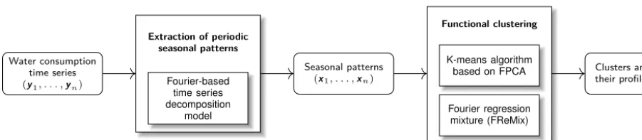
The aim of this paper is to identify automatically the major water usage patterns in a set of time series recorded by smart water meters. A multi-step methodology is formulated to ad-dress this problem, as illustrated in Fig. 1. The first step con-sists in extracting the seasonal part of each time series, which represents the habits of water consumption for each meter,
extraction and clustering approaches are described in the next sections.
3 Extracting seasonal patterns from time series
Let (y1, . . .,yn) denote n time series, where each one of them, yi=(yi1, . . ., yiT), corresponds to hourly
consump-tions recorded by a single water meter, that is to say,yi is a univariate time series andyit is a real-valued scalar. It is
implicitly assumed that all the series are recorded over the same time grid indexed by the ordered times{1, . . ., T}for allncurves.
3.1 Fourier-based time series decomposition
The methodology developed in this paper is based on the fol-lowing classical additive decomposition:
yit =fit+xit+dit+εit, (1)
where
– fit is the global trend of the time series which is
mod-eled in a nonparametric way using moving averages (Gourieroux et al., 1997), and
– xitis the seasonal component. As the studied water
con-sumption time series are subject to daily and weekly seasonality, a Fourier basis decomposition (De Livera et al., 2011) is formulated:
xit= q1
X
j=1
αj(1)cos
2πj t
24
+α(2)j sin
2πj t
24
+
q2
X
j=1
αj(3)cos
2πj t
168
+αj(4)sin
2πj t
168
, (2)
whereq1andq2are the respective numbers of
trigono-metric terms used to handle the daily and weekly sea-sonality, andαj(1),αj(2),α(3)j , andα(4)j are the coefficients to be estimated. This trigonometric modeling has the advantage of requiring considerably fewer parameters compared to an approach based on dummy variables (De Livera et al., 2011).
– dit is a component devoted to capturing the effect of
Figure 1.Block diagram describing the global methodology.
1 January, 1 May, Christmas Day). The following de-composition is used:dit =P24j=1γjδtj, whereδtj =1 if
t corresponds to the hourj of a non-working day and δtj=0 otherwise.
– εit is a centered Gaussian noise.
For compliance with the additivity and Gaussianity as-sumptions of this decomposition model, each time series (yit)t=1,...,T was replaced by (log(yit+λ))t=1,...,T, whereλ
is a small positive number preventing degeneracy caused by null consumptions. Note that this transformation is used in the same way as the well-known Box–Cox transformation (Box and Cox, 1964).
3.2 Parameter estimation and practical use of the model
Given a time seriesyi recorded by a smart meter, the trend
fi is estimated using a simple moving average (Gourieroux et al., 1997; Shumway and Stoffer, 2010). As the daily and weekly periodicities (24 and 168) should be removed from the univariate time series, a centered moving average of order 168 is performed.
After estimating the trend and given a couple (q1, q2), the
coefficients α1j, α2j, α3j, α4j and γj are simultaneously
identified by performing a multiple linear regression of (yit−
fit) over the variables cos 2πj t
24
, sin2πj t24 , cos2πj t168,
sin
2πj t
168
andδtj. Selecting the couple (q1, q2) remains a
sensitive point which can ideally be addressed by choos-ing the couple which optimizes a model selection criterion such as the Akaike information criterion (AIC) introduced by Akaike (1974) or the Bayesian information criterion (BIC) introduced by Schwarz (1978). In this paper, several combi-nations of (q1, q2) were tested and the couple (4,24) has been
selected, leading to a good compromise between visual rep-resentation of seasonal patterns and modeling accuracy. An example of decomposition of a time series is shown in Fig. 2. The trend is displayed together with the complete time series, while the seasonal component is displayed with the weekly sub-series.
From each time seriesyi, the model parameters defined by Eq. (1) are thus identified, and the periodic seasonal pattern defined by xi=(xi1, . . ., xim), with m=168, is extracted.
Due to the periodicity of the series (xit, . . ., xiT) defined by
Eq. (2), it should be noted that the first termsm=168 are sufficient to characterize the time series. Then, the set of seasonal patterns (x1, . . .,xn) is standardized as suggested
by Gaffney (2004):xit ←
xit−(1/m)Pmj=1xij
σ(xi)
,∀i, t,where σ(xi) is the standard deviation ofxi. The set of normalized
seasonal patterns is used as input data for the clustering step which will be described in the following section.
It is worth noting that the proposed decomposition can also be used to fill missing values that may occur along the time series. The reconstruction formula isyˆit = ˆfit+ ˆxit+ ˆdit,
wherefˆit,xˆit, anddˆit are the estimated components.
4 Clustering seasonal profiles
In order to extract relevant usage profiles from water con-sumption time series, two functional data clustering ap-proaches are considered in this paper: the first one is the func-tional version of theK-means algorithm and the second one is based on a specific Fourier regression mixture model.
4.1 Functional clustering based on FPCA
In this subsection, the clustering method (Peng and Müller, 2008; Sood et al., 2009) is inspired by functional data analy-sis (Ramsay and Silverman, 2005; Wang et al., 2015) which assumes that data are functions or curves. This clustering ap-proach is mainly based on functional principal component analysis (FPCA) and can be summarized in the following two consecutive steps.
Smoothing and dimension reduction This step consists in converting thentime series (x1, . . .,xn) into functional
objects (x1(t), . . .,xn(t)) and then applying the
classi-cal PCA to the multivariate data obtained by discretiz-ing the functionsxi(t) over the temporal grid{1, . . ., m}.
In this paper, the PCA is directly performed on the sea-sonal patterns (x1, . . .,xn) that are based on
20 40 60 80 100 120 140 160 −2
0 2 4 6
MON TUE WED THU FRI SAT SUN
Time (hours)
Normalized
log−consumption
(b) Seasonal component
Detrended weekly time series Estimated seasonality
Figure 2.Extraction of periodic seasonal patterns using Fourier-based time series decomposition. The trend is displayed with the complete time series(a)and the seasonal component is displayed with the weekly time series(b).
Clustering in this step consists of a classical clustering method performed on the principal component scores estimated previously. The well-known K-means algo-rithm (MacQueen, 1967) is applied using several ran-dom initializations and the partition with the lowest intra-cluster inertia is selected.
The resulting functional clustering strategy is called FPCA-KM. The number of clusters K has been selected by minimizing the BIC-like penalized criterion BIC(K)=
C+νKlog(n), whereCis the intra-cluster inertia optimized
by the K-means algorithm and νK=Kq is the number of
parameters to be estimated with q the number of selected principal components.
The general idea of PCA is to create a small number of un-correlated variables with maximal variance. The extension of this technique for functional data is proposed in the work of Ramsay and Silverman (2005) and Ferraty and Vieu (2006). The FPCA is an efficient tool providing common functional components explaining the structures of individual trajecto-ries.
4.2 Fourier regression mixture model
Inspired by the polynomial regression mixture model formu-lated by Gaffney and Smyth (1999), this subsection intro-duces a Fourier regression mixture model, called the FReMix model. The Fourier regression mixture was preferred to poly-nomial and spline regression mixtures for its compliance with the modeling adopted in the first step (seasonal pattern extraction). Moreover, a Fourier polynomial is a universal approximator of functions and remains a good candidate in modeling clusters whose prototypes are nonlinear and poten-tially periodic functions.
4.2.1 Model definition
Unlike standard vector-based mixture models, the density of each component of the FReMix model is represented by a trigonometric prototype function that is parameterized by regression coefficients and a noise variance. The prototype functions represent the class conditional expectations ofxi.
The Fourier regression mixture model therefore assumes that each time seriesxi is distributed according to the following
density:
f(xi;θ)= K X
k=1
πkN
xi;Uβk, σk2I
, (3)
whereθ=(π1, . . ., πK,β1, . . .,βK, σ12, . . ., σK2) is the
com-plete parameter vector. The probabilities πk are the
pro-portions of the mixture satisfying PKk=1πk=1, βk=
(βk,1, . . ., βk,2(q1+q2)) 0∈
R2(q1+q2)is the coefficient vector of thekth regression model andσk2>0 is the associated noise variance. The matrixU=(u1, . . .,um)0 is a regression
ma-trix of sizem×2(q1+q2), where the vectorut∈R2(q1+q2)is defined by (∀t=1, . . ., m):
ut=
cos
2π t 24
sin
2π t
24
· · ·cos
2π q1t 24
sin
2π q1t
24
cos
2π t
168
sin
2π t
168
· · ·cos
2π q 2t
168
sin
2π q 2t
168
0
,
andN(·;µ,6) is the Gaussian density with mean vectorµ
which is also given by
gk(t)= q1
X
j=1
βk,2j−1cos 2πj t
24
+βk,2jsin 2πj t
24
+
q2
X
j=1
βk,2q1+2j−1cos
2πj t
168
+βk,2q1+2jsin
2πj t
168
. (4)
4.2.2 EM algorithm and practical issues
Assuming that the n seasonal time series (x1, . . .,xn)
are independent, the parameter vector θ is estimated in the same way as for the classical Gaussian mixture model (McLachlan and Krishnan, 2007) and the poly-nomial regression mixture model (Gaffney and Smyth, 1999), by maximizing the specific log-likelihood L(θ)=
Pn i=1log
PK
k=1πkN xi;Uβk, σk2I
via the EM procedure (Dempster et al., 1977; Gaffney and Smyth, 1999; McLach-lan and Krishnan, 2007). The pseudo-code can be found in the paper by Samé et al. (2016). As a reminder, the couple (q1, q2)=(4,24) is selected in the seasonal pattern extraction
step (cf. Sect. 3.2). The algorithm is initialized as follows: the initial regression coefficients and variances are obtained by performing a Fourier regression separately onKseasonal series randomly drawn into the data set (x1, . . .,xn) and the
initial proportions of the latent classes are set to πk=K1.
This process is repeated 20 times and the parameters with the highest log-likelihood are selected. The number of clusters is selected through the BIC criterion (Schwarz, 1978) defined by BIC(K)= −2L(θˆ)+νKlog(n), whereθˆis the parameter
vector estimated by the EM algorithm, andνKis the number
of free parameters of the model:νK=2K(q1+q2+1)−1.
After estimating the parameter vector θ, a time se-ries partition is obtained by assigning each sese-ries xi to
the cluster having the highest posterior probability τik= πkN xi;Uβk,σk2I
PK
`=1π`N xi;Uβ`,σ`2I ·
5 Experimental study using real data
5.1 Description of the data set
The experimental data set represents the water consumption recorded by a few smart meters deployed on the network of the Syndicat des Eaux d’Ile-de-France (SEDIF). The SEDIF is a large association including 150 municipalities which provides drinking water for more than 4 million inhabitants of suburban Paris. This is the largest drinking water distri-bution network (WDN) in France, with about 8000 km of pipes and more than 750 000 m3of water produced each day. The consumption is measured hourly (in liters) by 10 233 m during 15 months (from November 2013 to March 2015). The resulting data set is then made of univariate time
se-0 2 4 6 8 10 12 14 16 18 20
1.5 2 2.5 3 3.5 4 4.5x 10
4
Number of clusters
BIC criterion
FReMix (x0.2) FPCA−KM
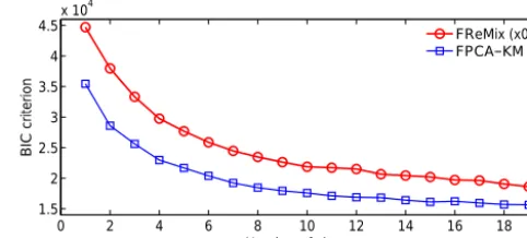
Figure 3.Evolution of the BIC criteria according to the number of clusters.
ries (y1, . . .,yn), where n=10 233 and the length of each time series yi is T =11 016. After the extraction of peri-odic seasonal patterns (cf. Sect. 3), a new set of time series (x1, . . .,xn) is built where the length of each seasonal pattern xi is m=168. These series are used as input data for the clustering algorithms.
5.2 Selecting the number of clusters
The number of clusters for the two methods was selected by running the algorithms with several values of K and then choosing the value which minimizes the BIC criterion. Fig-ure 3 shows the evolution of this criterion for the two cluster-ing algorithms in relation to the number of clusters. For both methods, the BIC criterion exhibits a decrease continuously, while theKvalue increases. Nevertheless, it can be seen that the variation of BIC is not significant when the number of clusters is above eight. Therefore, the number of clusters is selected such thatK=8.
5.3 Results interpretation and discussion
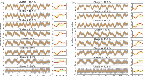
The seasonal time series are classified intoK=8 clusters, using functionalK-means (FPCA-KM strategy) and Fourier regression mixture (FReMix model) as illustrated, respec-tively, by Fig. 4a and b. For each cluster, the weekly pro-totype is displayed in orange (sub-figures on the left). More-over, the right plots of Fig. 4a and b display the cluster pro-files using a daily representation, the colors (from blue to red) indicating the day of the week (from Monday to Sun-day). The percentage of input time series belonging to each cluster is also provided.
It can be observed that the consumption profiles are quite similar for the two methods, despite the differences in the cluster percentages. As no socio-demographic data about customers were available at this stage of the study, a qual-itative evaluation of the results is performed and the pattern repartition shown in Fig. 4 can be explained by the following realistic categories.
Figure 4.Clustering results obtained with the FPCA-KM(a)and the FReMix(b). For each side, the subfigures on the left represent a weekly view of the clusters with their prototypes displayed in orange. The subfigures on the right are daily prototypes resulting from the segmentation of the weekly orange curves and colors (from blue to yellow to red) indicate the day of the week (from Monday to Sunday).
between 06:00 and 08:00, take a shower and then go to work. This habit is characterized by a consumption peak around 10:00 in the morning. The other peak, observed in the evening at around 20:00, corresponds to the return home. The minimum consumption level between these two peaks can be attributed to persons in households who stay at home during working hours.
Commercial use Clusters 4,5, and 6. This category corre-sponds to a set of customers whose consumption habits are the same during working days and weekends. It may correspond, for example, to small businesses or medical centers that stay open every day and have the same daily consumption profile. It should be noticed that clusters 4 and 5 differ from the other clusters by their smaller evening peak.
Office or industrial use Cluster 7. One can observe an ac-tive water consumption from Monday to Friday (work-days) during the business hours, and a very low con-sumption during the weekend.
Noise cluster Cluster 8. This cluster, which has the largest variance, groups a set of atypical patterns which does not match with the other clusters. It can be considered a noise cluster.
Note that a functional clustering scheme is adopted be-cause this is suitable for dealing with the analysis of our
con-sumption curves. Indeed, these real-valued data can be seen as the realizations of a one-dimensional stochastic process, recorded on the same time grid (hourly spaced) of ordered times. In practice, data frames are frequently sent by modules which are physically connected to the meters; each consump-tion time series can be re-constructed based on a sequence of the data frames. Exogenous variables (e.g., weather inputs or meter localization) are not considered in this work due to a non-significant improvement in the results, but might be used in a future work.
Furthermore, the time seriesxi have a length of 168 due
to the trigonometric modeling of the chosen Fourier basis de-composition. The Fourier coefficients are identified by per-forming a multiple linear regression on the detrended global time seriesyi, which limits the effect of a long seasonality. Finally, our sample has a duration of 15 months (with five seasons at most), and we are more interested in identifying the major mode of consumption than estimating water de-mand profiles with local changes and a fine granularity.
might not be straightforward and the number of parameters in this case should not be reduced significantly. In this ar-ticle, we evaluate a probabilistic method and a geometrical approach. This second method is based on a K-means and minimizes the intra-cluster inertia which can be seen as an aggregated distance over the water time series. To our knowl-edge, the complexity of time series distances (e.g., dynamic time warping) can be prohibitive with a large time series data set.
This paper deals with an unsupervised classification prob-lem based on water consumption time series. Water demand forecasting is not the issue in this paper; nevertheless, the re-sulting segmentation of water consumption time series can be used for several scientific problems, including sequential de-tection, predictive classification or demand forecasting. We assume no supervision in our setting due to a partial and un-certain knowledge of the usage labels; users do not inform systematically their water utilities when businesses change or people come in/leave a home. This is why there is no quanti-tative accuracy about clustering. Each log-consumption time series is standardized before clustering, which leads to a dis-crimination in terms of seasonal patterns and is not based on water volume. This explains why we called cluster 1 “of-fice and industrial usage”. Of course, industrial usage might produce erratic water patterns which would be classified in cluster 2. Partitioning the eight clusters into four categories would suggest non-negligible variations in residential use as well as commercial use, and extra investigations about the users which should not be underestimated in terms of time and cost. The EM algorithm used to fit the Fourier REgres-sion Mixture (FReMix) model is flexible and can be refor-mulated in a future work with a semi-supervision (by fixing a set of posterior probabilities) or a partial supervision (e.g., using belief functions).
Identifying the major usage profiles from water consump-tion is an interesting topic to water utilities. Indeed, the re-sulting segmentation helps the water companies to gain bet-ter knowledge about users consuming the distributed wabet-ter. The user has a better experience with the tools developed by their water utility. For instance, users at Veolia Eau d’Ile de France (Paris area in France) can already monitor their wa-ter index/consumption on a dedicated website for free. Using our clustering results, people could compare with similar pat-terns and adapt their consumptions according to their needs. In addition, the resulting clusters are used by an early warn-ing system which alerts the user when a leakage occurs into the private network. An erratic water pattern (like in cluster 2) can be a sign of a leakage and might initiate a corrective action. Concerning the grid management, each prototype can be used to represent the water behavior of users belonging to the same cluster. Sampling a large amount of water meters is useful for several topics (e.g., tracking the meter metrology, estimating the global consumption modes based on a limited number of meters); such sampling analysis is straightforward using our meter segmentation.
6 Conclusions and perspectives
A general methodology is introduced in this paper for au-tomatically discriminating several water usages and extract-ing relevant water consumption profiles from time series recorded by smart meters. Considering that the consumption habits are of interest and not the consumption levels, the first step of the method consists in extracting the seasonal part of time series using an additive classical decomposition model. This modeling of the seasonal component is based on a spe-cific Fourier expansion which takes into account daily and weekly periodicities. As this study aims to identify relevant water usage profiles, two functional clustering techniques are used to classify the seasonal patterns extracted from the wa-ter consumption time series: a functional variant of theK -means algorithm and a specific EM algorithm based on a Fourier regression mixture model (FReMix). The FReMix model is richer than the other clustering approach in that the Fourier basis decomposition is fully integrated in the mod-eling and each cluster is described by its first two moments, while theK-means only extracts the mean curves. Further-more, theK-means produces a hard segmentation, while the FReMix creates a soft partition where each cluster member-ship is weighted by a posterior probability. Eight clusters are then identified for the two clustering methods. The resulting prototypes are quite similar for the two approaches and a re-alistic category is given to each cluster.
More investigations are in progress with the water utility Veolia Eau d’Ile de France in order to refine the clustering results and the proposed methodology is also being applied to a new large-scale database.
Data availability. The data set is private and belongs to the SEDIF.
Competing interests. The authors declare that they have no con-flict of interest.
Special issue statement. This article is part of the special issue “Computing and Control for the Water Industry, CCWI 2016”. It is a result of the 14th International CCWI Conference, Amsterdam, the Netherlands, 7–9 November 2016.
Acknowledgements. The study presented in the paper was part of a previous work between IFSTTAR and Veolia Eau d’Ile de France. This work is now part of French–German collaborative research project ResiWater (http://www.resiwater.eu/) that is funded by the French National Research Agency (ANR; project: ANR-14-PICS-0003) and the German Federal Ministry of Educa-tion and Research (BMBF; project: BMBF-13N13690).
Edited by: Edo Abraham
137, 456–467, 2010.
Blokker, E., Vreeburg, J., and Van Dijk, J.: Simulating residential water demand with a stochastic end-use model, J. Water Res. Pl.-ASCE, 136, 19–26, 2009.
Box, G. E. and Cox, D. R.: An analysis of transformations, J. Roy. Stat. Soc. B, 211–252, 1964.
Cardell-Oliver, R.: Water use signature patterns for analyzing household consumption using medium resolution meter data, Water Resour. Res., 49, 8589–8599, 2013.
Cheifetz, N., Samé, A., Aknin, P., De Verdalle, E., and Chenu, D.: A Sequential Testing Procedure for Multiple Change-Point De-tection in a Stream of Pneumatic Door Signatures, in: 12th In-ternational Conference on Machine Learning and Applications (ICMLA), IEEE, 117–122, 2013.
Dabo-Niang, S., Ferraty, F., and Vieu, P.: On the using of modal curves for radar waveforms classification, Comput. Stat. Data An., 51, 4878–4890, 2007.
De Livera, A. M., Hyndman, R. J., and Snyder, R. D.: Forecast-ing time series with complex seasonal patterns usForecast-ing exponential smoothing, J. Am. Stat. Assoc., 106, 1513–1527, 2011. Dempster, A. P., Laird, N. M., and Rubin, D. B.: Maximum
likeli-hood from incomplete data via the EM algorithm, J. Roy. Stat. Soc. B, 1–38, 1977.
Donkor, E. A., Mazzuchi, T. A., Soyer, R., and Alan Roberson, J.: Urban water demand forecasting: review of methods and models, J. Water Res. Pl.-ASCE, 140, 146–159, 2012.
Ferraty, F. and Vieu, P.: Nonparametric Functional Data Analy-sis: Theory and Practice (Springer Series in Statistics), Springer-Verlag New York, Inc., 2006.
Gaffney, S. and Smyth, P.: Trajectory clustering with mixtures of regression models, in: Proceedings of the fifth ACM SIGKDD international conference on Knowledge discovery and data min-ing, ACM, 63–72, 1999.
Gaffney, S. and Smyth, P.: Curve Clustering with Random Effects Regression Mixtures, in: Proceedings of the Ninth International Workshop on Artificial Intelligence and Statistics (AISTATS), 2003.
Gaffney, S. J.: Probabilistic curve-aligned clustering and prediction with regression mixture models, PhD thesis, University of Cali-fornia, Irvine, 2004.
Giffinger, R., Fertner, C., Kramar, H., Kalasek, R., Pichler-Milanovic, N., and Meijers, E.: Smart Cities – Ranking of Eu-ropean medium-sized cities, Vienna University of Technology, 2007.
Jacques, J. and Preda, C.: Model-based clustering for multivariate functional data, Comput. Stat. Data An., 71, 92–106, 2014. MacQueen, J.: Some methods for classification and analysis of
mul-tivariate observations, in: Proceedings of the fifth Berkeley sym-posium on mathematical statistics and probability, Oakland, CA, USA, 1, 281–297, 1967.
McKenna, S., Fusco, F., and Eck, B.: Water demand pattern classi-fication from smart meter data, Procedia Engineering, 70, 1121– 1130, 2014.
McLachlan, G. and Krishnan, T.: The EM algorithm and extensions, 382, John Wiley & Sons, 2007.
Nam, T. and Pardo, T. A.: Conceptualizing smart city with dimen-sions of technology, people, and institutions, in: Proceedings of the 12th annual international digital government research confer-ence, ACM, 282–291, 2011.
Peng, J. and Müller, H.-G.: Distance-based clustering of sparsely observed stochastic processes, with applications to online auc-tions, The Annals of Applied Statistics, 1056–1077, 2008. Ramsay, J. O. and Silverman, B. W.: Functional Data Analysis,
Springer Series in Statistics, Springer, 2nd Edn., 2005.
Samé, A., Chamroukhi, F., Govaert, G., and Aknin, P.: Model-based clustering and segmentation of time series with changes in regime, Advances in Data Analysis and Classification, 5, 301– 321, 2011.
Samé, A., Noumir, Z., Cheifetz, N., Sandraz, A.-C., and Féliers, C.: Décomposition et classification de données fonctionnelles pour l’analyse de la consommation d’eau potable (in french), in: Ex-traction et Gestion des Connaissances (EGC) conference – Clus-tering and Co-clusClus-tering (CluCo) workshop, 2016.
Schwarz, G.: Estimating the dimension of a model, Ann. Stat., 6, 461–464, 1978.
Shumway, R. H. and Stoffer, D. S.: Time series analysis and its ap-plications: with R examples, Springer Science & Business Me-dia, 2010.
Sood, A., James, G. M., and Tellis, G. J.: Functional regression: A new model for predicting market penetration of new products, Marketing Science, 28, 36–51, 2009.