Estimating the Reliability Function of (2+1) Cascade Model

Baghdad Science Journal

Vol.16(2)2019

Estimating the Reliability Function of (2+1) Cascade Model

Ahmed H. Khaleel

Nada S. Karam

Received 20/5/2018, Accepted 20/12/2018, Published 2/6/2019

This work is licensed under a Creative Commons Attribution 4.0 International License.

Abstract:

This paper discusses reliability R of the (2+1) Cascade model of inverse Weibull distribution. Reliability is to be found when strength-stress distributed is inverse Weibull random variables with unknown scale parameter and known shape parameter. Six estimation methods (Maximum likelihood, Moment, Least Square, Weighted Least Square, Regression and Percentile) are used to estimate reliability. There is a comparison between six different estimation methods by the simulation study by MATLAB 2016, using two statistical criteria Mean square error and Mean Absolute Percentage Error, where it is found that best estimator between the six estimators is Maximum likelihood estimation method.

Key words: Attenuation factor, Least Square, Scale parameter, Simulation, Strength-Stress .

Introduction:

In standby systems one component work's and the other components are standby. Cascade is a special kind of strength and stress reliability model. Special (2+1) of cascade model contain three components (comp1, comp2 and comp3), where comp1 and comp2 are activate while comp3 remains standby. Suppose that X1, Y1 indicate the

strength and stress of comp1 and X2, Y2 indicate the

strength and stress of comp2. Now, if comp1 or comp2 fail's the standby component (comp3) is activated. Let X3, Y3 indicate the strength and stress

of comp3. Now, if comp1 fail's: X3= mX1 and

Y3= kY1 and if comp2 fail's: X3= mX2 and

Y₃= kY₂ , where (m) is stress attenuation factor and (k) is strength attenuation factor and (0 < 𝑚 < 1 ,

𝑘 > 1) .

Ozler and Gurler (2012) (1) considered reliability of the k-out-of-n: F systems and its conditional shape with exchangeable components in stress-strength setup. Gogoi and Borah (2012) (2) studied two cases to obtain system reliability for the cascade model. Sandhya and Umamaheswari (2013) (3) worked on a multi-unit standby the model of strength and stress. Umamaheswari and Swathi (2013) (4) studied generalized exponential distribution for cascade model. Singh (2013) (5) considered n of cascade model by strength is exponential distribution and stress is normal

1_{Department of Statistics, College of Administration &} Economics, University of Sumer, Dhi Qar, Iraq

2 _{Department of Mathematics, College of Education,} Al-Mustansiriyah University, Baghdad, Iraq

* _{Corresponding author: [email protected]}

distribution to find reliability. Reddy (2016)(6) presented estimation of R = (X > Y) by considering the cascade stress-strength model. Devi, Umamaheswari and Swathi (2016) (7) studied general expression for reliability by n cascade system is derivative when stress and strength follow the lindley distribution and numerical values

R₍₁₎ , R₍₂₎ , R₍₃₎ and R₃ have been computed for the some specific values of parameters. Mutkekar and Munoli (2016) (8) endeavored to the (1 + 1) cascade model by exponential distribution under joint action of stress strength. Karam and Husieen (2017) (9) studied n cascade model while strength-stress are Frechet distributed r.v to find the reliability, and used Marginal Reliabilities values of cascade model to find the reliabilities

R2, R3 and R4. Karam and Khaleel (2018) (10)

discussed reliability (2+1) cascade model where strength and stress are WD, and used (Maximum likelihood, Moment, Least Square and Weighted Least Square) methods to estimate reliability of this model.

The Mathematical Formula Reliability:

In this model strength-stress random variables of (comp1 and comp2 are basics and comp3 is stand by) to be (𝑋𝑖; 𝑖 = 1,2,3) and (𝑌𝑗; 𝑗 = 1,2,3)

respectively , where 𝑋𝑖 and 𝑌𝑗 are independently

identically distributed Inverse Weibull random variables with common known shape parameter 𝜎 and unknown scale parameters ρi; i=1,2,3 , θj;

j=1,2,3 .

The CDF of IW(σ, ρ) is :

𝐹(𝑥) = 𝑒−𝜌𝑥−𝜎

𝑥 > 0; 𝜎, 𝜌 > 0 …..(1) The PDF of IW(σ, ρ) is :

𝑓(𝑥) = 𝜎𝜌𝑥−(𝜎+1)_𝑒−𝜌𝑥−𝜎

𝑥 > 0; 𝜎, 𝜌 > 0 …..(2) and

The CDF of IW(σ, θ) is :

𝐺(𝑦) = 𝑒−𝜃𝑦−𝜎 _{𝑦 > 0; 𝜎, 𝜃 > 0 …..(3)}

The PDF of IW(σ, θ) is :

𝑔(𝑦) = 𝜎𝜃𝑦−(𝜎+1)_𝑒−𝜃𝑦−𝜎 _{𝑦 > 0; 𝜎, 𝜃 > 0 …..(4)}

Reliability function R for (2+1) the cascade model:

𝑅 = 𝑝[𝑋₁≥ 𝑌₁, 𝑋₂≥ 𝑌₂] + 𝑝[𝑋₁< 𝑌₁, 𝑋₂≥ 𝑌₂, 𝑋₃≥ 𝑌₃] + 𝑝[𝑋1≥ 𝑌1, 𝑋2< 𝑌2, 𝑋3≥ 𝑌3]

𝑅 = 𝑅₁+ 𝑅₂+ 𝑅₃ …..(5)

𝑅₁= 𝑝[𝑋₁≥ 𝑌₁, 𝑋₂ ≥ 𝑌₂]

= ∫ 𝑝[𝑋₀∞ 1≥ 𝑌1]𝑔(𝑦1)𝑑𝑦1∫ 𝑝[𝑋₀∞ 2≥ 𝑌2]𝑔(𝑦2)𝑑𝑦2 = ∫ [∫ 𝑓(𝑥₀∞ _𝑦∞₁ 1)𝑑𝑥1] 𝑔(𝑦1)𝑑𝑦1∫ [∫ 𝑓(𝑥₀∞ _𝑦∞₂ 2)𝑑𝑥2] 𝑔(𝑦2)𝑑𝑦2

= ∫ [𝐹𝑥1(𝑦1)]𝑔(𝑦1)𝑑𝑦1∫ [𝐹𝑥2(𝑦2)]𝑔(𝑦2)𝑑𝑦2 ∞

0 ∞

0

= ∫ [1 − 𝑒∞ −𝜌1𝑦1−𝜎_{]𝜎𝜃1𝑦1}−(𝜎+1)_𝑒−𝜃1𝑦1−𝜎_𝑑𝑦1 0

.∫ [1 − 𝑒∞ −𝜌2𝑦2−𝜎_{]𝜎𝜃2𝑦2}−(𝜎+1)_𝑒−𝜃2𝑦2−𝜎_𝑑𝑦2 0

Then it becomes as

𝑅1= [_𝜌𝜌1 1+𝜃1] [

𝜌2

𝜌2+𝜃2] ….(6)

For R2 we have that :

𝑅₂= 𝑝[𝑋₁< 𝑌₁, 𝑋₂≥ 𝑌₂, 𝑋₃≥ 𝑌₃] = 𝑝[𝑋1<

𝑌₁, 𝑚𝑋₁ ≥ 𝑘𝑌₁]𝑝[𝑋₂ ≥ 𝑌₂] Where from above we have that:

𝑝[𝑋₂≥ 𝑌₂] = ∫ (𝐹𝑥2(𝑦2)) 𝑔(𝑦2)𝑑𝑦2= [ 𝜌2 𝜌2+𝜃2] ∞

0

and

p[X1< Y1, mX1≥ kY1] = ∫ (Fx1(y1)) ∞

0 (Fx1( k my1))

g(y1)dy1

= ∫ [e∞ −ρ1y1−σ_]

0 [1 − e

−𝛒1(_mky1)−σ_]

σ1θ1y1−(σ+1)e−θ1y1 −σ dy1 = [ ( k m) −σ ρ1θ1

(ρ1+(_mk)−σρ1+θ1)(ρ1+θ1)]

So

R₂= [ (

k m)

−σ ρ1θ1

(ρ1+(_mk)−σρ1+θ1)(ρ1+θ1)] [ ρ2

ρ2+θ2] …..(7)

By using the same steps above we can find R3 :

𝑅3= 𝑝[𝑋1≥ 𝑌1, 𝑋2< 𝑌2, 𝑋3≥ 𝑌3] =

= [_𝜌𝜌1

1+𝜃1] [

(_𝑚𝑘)−𝜎𝜌2𝜃2

(𝜌2+(_𝑚𝑘) −𝜎

𝜌2+𝜃2)(𝜌2+𝜃2)

] …..(8)

substitution (6),(7) and ,(8) in (5)the reliability function; R, finally will be as:

𝑅 = [ 𝜌1

𝜌₁+𝜃₁] [ 𝜌2 𝜌₂+𝜃₂] + [

(_𝑚𝑘)−𝜎𝜌1𝜃1

(𝜌₁+(_𝑚𝑘)−𝜎𝜌₁+𝜃₁)(𝜌₁+𝜃₁)] [ 𝜌2 𝜌₂+𝜃₂]

+ [ 𝜌1 𝜌₁+𝜃₁] [

(_𝑚𝑘)−𝜎𝜌2𝜃2

(𝜌₂+(_𝑚𝑘)−𝜎𝜌₂+𝜃₂)(𝜌₂+𝜃₂)] ….(9)

Methods of Estimating the Reliability Function

Maximum likelihood Estimation method (ML): Let 𝑥1, 𝑥2, … , 𝑥𝑛 a random sample from

IW(σ, ρ) distribution. The general form is: 𝐿(𝜎, 𝜌; 𝑥1, 𝑥2, … 𝑥𝑛) = (𝜎𝜌)𝑛∏ 𝑥𝑖

−(𝜎+1) 𝑛

𝑖=1 𝑒−𝜌 ∑ 𝑥𝑖 −𝜎 𝑛 𝑖=1

….(10) The log - equation (10) :

𝐿𝑛𝐿 = 𝑛𝐿𝑛(𝜎) + 𝑛𝐿𝑛(𝜌) − (𝜎 + 1) ∑𝑛𝑖=1𝑙𝑛(𝑥𝑖)

−𝜌 ∑𝑛_𝑖=1𝑥_𝑖−𝜎 …..(11) Taking partial derivative equation (11) :

𝜕 𝑙𝑛 𝐿(𝜎,𝜌; 𝑥1,𝑥2,…,𝑥𝑛)

𝜕𝜌 = 𝑛 𝜌− ∑ 𝑥𝑖 −𝜎 𝑛 𝑖=1

Then the maximum likelihood estimator for ρ is :

𝜌̂(𝑀𝐿) =_∑ 𝑛_𝑥 𝑖 −𝜎 𝑛

𝑖=1 …..(12)

By using the same manner, we can obtain the maximum likelihood estimators for the unknown scale parameters ρ1, ρ2, ρ3 of the strength random

variables X₁∼ IW(σ, ρ₁), X₂∼ IW(σ, ρ₂), X₃ ∼

IW(σ, ρ₃) with sample sizes n1 , n2and n3,

respectively, and θ1, θ2, θ3 to the stress random

variables Y₁∼ IW(σ, θ₁), Y₂ ∼ IW(σ, θ₂), Y ∼

IW(σ, θ₃) with sample sizes m1 , m2and m3 then

the formulas will be as

𝜌̂𝜉(𝑀𝐿) = 𝑛𝜉 ∑ 𝑥 𝜉𝑖𝜉 −𝜎 𝑛𝜉 𝑖𝜉=1

,𝜉 = 1,2,3 …..(13)

and 𝜃̂𝜉(𝑀𝐿) = 𝑚𝜉 ∑ 𝑦 𝜉𝑗𝜉−𝜎 𝑚𝜉 𝑗𝜉=1

, ξ = 1,2,3 ……(14)

Substitution (13) and (14) in (9),the ML estimator for reliability R ; says R̂_(ML) :

𝑅̂(𝑀𝐿)= [_𝜌̂ 𝜌̂1(𝑀𝐿) 1(𝑀𝐿)+𝜃̂1(𝑀𝐿)] [

𝜌 ̂2(𝑀𝐿) 𝜌

̂2(𝑀𝐿)+𝜃̂2(𝑀𝐿)]

+ [ (

𝑘 𝑚)

−𝜎 𝜌

̂_1(𝑀𝐿)𝜃̂1(𝑀𝐿)

(𝜌̂1(𝑀𝐿)+(_𝑚𝑘) −𝜎

𝜌̂1(𝑀𝐿)+𝜃̂1(𝑀𝐿))(𝜌̂1(𝑀𝐿)+𝜃̂1(𝑀𝐿))

] [ 𝜌̂2(𝑀𝐿) 𝜌̂2(𝑀𝐿)+𝜃̂2(𝑀𝐿)]

+ [ 𝜌̂1(𝑀𝐿) 𝜌

̂1(𝑀𝐿)+𝜃̂1(𝑀𝐿)] [

(_𝑚𝑘)−𝜎𝜌̂2(𝑀𝐿)𝜃̂2(𝑀𝐿)

(𝜌̂_2(𝑀𝐿)+(_𝑚𝑘)−𝜎𝜌̂_2(𝑀𝐿)+𝜃̂_2(𝑀𝐿))(𝜌̂_2(𝑀𝐿)+𝜃̂_2(𝑀𝐿))] …..(15)

Moment Estimation method (Mo): In this method of IW(σ, ρ):

E(x) = ρ1σΓ (1 −1

σ) .….(16)

According to the method of moment ,equating the samples means with the corresponding populations mean

∑𝑛𝑖=1𝑥𝑖

𝑛 = 𝜌̂

1

𝜎𝛤 (1 −1

𝜎) …..(17)

𝜌̂_(𝑀𝑜)= [ 𝑥̅

𝛤(1−1_𝜎)] 𝜎

for σ > 1 ….. (18)

The Mo estimators of unknown scale parameters

(𝜌1, 𝜌2 , 𝜌3) and (𝜃1, 𝜃2 , 𝜃3) are :

𝜌̂_{𝜉(𝑀𝑜)}= [ 𝑥̅𝜉 𝛤(1−1_𝜎)]

𝜎

,ξ = 1,2,3 …..(19)

and

𝜃̂_{𝜉(𝑀𝑜)}= [ 𝑦̅𝜉 𝛤(1−1_𝜎)]

𝜎

,ξ = 1,2,3 …..(20)

Substitution (19) and (20) in (9),the Mo estimator for reliability R ; says R̂_(Mo) :

R

̂_{(Mo)= [} ρ̂1(Mo) ρ̂1(Mo)+ θ̂1(Mo)] [

ρ̂2(Mo) ρ̂2(Mo)+ θ̂2(Mo)]

+ [ ( k m)

−σ

ρ̂1(Mo)θ̂1(Mo) (ρ̂1(Mo)+(_mk)

−σ

ρ̂1(Mo)+θ̂1(Mo))(ρ̂1(Mo)+θ̂1(Mo))

] [ ρ̂2(Mo) ρ̂2(Mo)+θ̂2(Mo)]

+ ⌈_ρ̂ ρ̂1(Mo) 1(Mo)+θ̂1(Mo)⌉ [

(k m)

−σ

ρ̂2(Mo)θ̂2(Mo)

(ρ̂2(Mo)+(_mk) −σ

ρ̂2(Mo)+θ̂2(Mo))(ρ̂2(Mo)+θ̂2(Mo))

]

…..(21)

Least Square Estimation Method (LS):

In least square method the minimize function of

IW(σ, ρ) :

𝑆(𝜎, 𝜌) = ∑ (𝐹̂(𝑥_𝑖) − 𝐹(𝑥𝑖)) 2 𝑛 𝑖=1 = ∑ (𝐹̂(𝑥𝑖) − 𝑒−𝜌𝑥 −𝜎 )2 𝑛

𝑖=1 …..(22)

Since CDF ofinverse Weibull distributiondoes not have a linear formula giving to the parameters, so we get the linear formula the following :

𝐹(𝑥𝑖) = 𝑒−𝜌𝑥𝑖 −𝜎

−𝑙𝑛(𝐹(𝑥𝑖)) = 𝜌𝑥𝑖−𝜎 ……(23)

Since F̂(x_i) is unknown, so we use (11) :

𝐹̂(𝑥(𝑖)) =_𝑛+1𝑖

𝑆(𝜎, 𝜌) = ∑𝑛_𝑖=1(𝑞_(𝑖)− 𝜌𝑥_(𝑖)−𝜎)2 ……(24) Where 𝑞_(𝑖)= −𝑙𝑛 (𝐹̂(𝑥_(𝑖))) = −𝑙𝑛(𝑃_𝑖) and 𝑃_𝑖is the plotting position

By derivative equation (24) with respect to parameter 𝜌 (12) :

𝜕𝑆(𝜎,𝜌)

𝜌 = ∑ 2(𝑞(𝑖)− 𝜌𝑥(𝑖)

−𝜎₎ 𝑛

𝑖=1 𝑥(𝑖)−𝜎

∑𝑛 𝑞_(𝑖)𝑥_(𝑖)−𝜎

𝑖=1 − 𝜌 ∑𝑛𝑖=1𝑥(𝑖)−2𝜎= 0

Then we get the least square estimator of ; say

𝜌̂_(𝐿𝑆):

𝜌̂_(𝐿𝑆)=∑𝑛𝑖=1𝑞(𝑖)𝑥(𝑖)−𝜎 ∑𝑛 𝑥_(𝑖)−2𝜎

𝑖=1 …..(25)

The LS estimators of unknown scale parameters

(𝜌1, 𝜌2 , 𝜌3) and (𝜃1, 𝜃2 , 𝜃3) are :

𝜌̂_{𝜉(𝐿𝑆)}= ∑ 𝑞𝜉 (𝑖𝜉)𝑥𝜉(𝑖𝜉) −𝜎 𝑛𝜉 𝑖𝜉=1 ∑ 𝑥_𝜉 (𝑖𝜉) −2𝜎 𝑛𝜉 𝑖𝜉=1 ……(26) and 𝜃̂𝜉(𝐿𝑆) = ∑ 𝑞𝜉 (𝑗𝜉)𝑦𝜉(𝑗𝜉) −𝜎 𝑚𝜉 𝑗𝜉=1 ∑ 𝑦_𝜉 (𝑗𝜉) −2𝜎 𝑚𝜉 𝑗𝜉=1 ……(27)

Where 𝐺̂(𝑦_(𝑗)) =_𝑚+1𝑗 and

𝑞_(𝑗) = −𝑙𝑛 (𝐺̂(𝑦(𝑗))) = −𝑙𝑛(𝑃𝑗)

Substitution (26) and (27) in (9),the LS estimator for reliability R ; says 𝑅̂(𝐿𝑆) :

R̂(LS)= [_ρ̂ ρ̂1(LS) 1(LS)+θ̂1(LS)] [

ρ̂_2(LS)

ρ̂_2(LS)+θ̂_2(LS)]

+ [ (

k m)

−σ

ρ̂_1(LS)θ̂_1(LS)

(ρ̂_1(LS)+(_mk)−σρ̂_1(LS)+θ̂_1(LS))(ρ̂_1(LS)+θ̂_1(LS))] [ ρ̂_2(LS) ρ̂_2(LS)+θ̂_2(LS)]

+ ⌈ ρ̂1(LS) ρ̂_1(LS)+θ̂_1(LS)⌉ [

(_mk)−σρ̂_2(LS)θ̂_2(LS)

(ρ̂_2(LS)+(_mk)−σρ̂_2(LS)+θ̂_2(LS))(ρ̂_2(LS)+θ̂_2(LS))]

…..(28) Weighted Least Square Estimation Method (WLS):

In this method we can use the minimizing equation to find estimator of unknown scale parameter of IWD [1] :

𝑆 = ∑ 𝑤𝑖(𝐹̂(𝑥𝑖) − 𝐹(𝑥𝑖)) 2 𝑛

𝑖=1 ..…(29)

Where 𝑤_𝑖 =_{𝑉𝑎𝑟[𝐹(𝑥}1 _𝑖)]=(𝑛+1)

2_(𝑛+2)

𝑖(𝑛−𝑖+1) , 𝑖 = 1,2, … , 𝑛

As steps in equations (23) and (24) we get :

𝑆 = ∑ 𝑤𝑖(𝑞(𝑖)− 𝜌𝑥(𝑖)−𝜎) 2 𝑛

𝑖=1 .….(30)

By derivative equation (30) :

𝜕𝑆

𝜕𝜌= ∑ 2𝑤𝑖(𝑞(𝑖)− 𝜌𝑥(𝑖)

−𝜎_)𝑥

(𝑖)−𝜎 𝑛

𝑖=1

∑𝑛 𝑤_𝑖𝑞_(𝑖)𝑥_(𝑖)−𝜎−

𝑖=1 𝜌̂ ∑𝑛𝑖=1𝑤𝑖𝑥(𝑖)−2𝜎= 0

Then we get the weighted least square estimator of

ρ ; say ρ̂(WLS):

𝜌̂_{(𝑊𝐿𝑆)}=∑𝑛𝑖=1𝑤𝑖𝑞(𝑖)𝑥(𝑖)−𝜎

∑𝑛𝑖=1𝑤𝑖𝑥(𝑖)−2𝜎 …..(31)

The WLS estimators of unknown scale parameters

(𝜌1, 𝜌2 , 𝜌3) and (𝜃1, 𝜃2 , 𝜃3) are :

ρ̂_ξ(WLS)=

∑ w_iξqξ

(iξ)xξ(iξ) −σ nξ

iξ=1

∑ w_iξx_ξ

(iξ) −2σ nξ

iξ=1

,ξ = 1,2,3 …..(32)

and

θ̂_ξ(WLS)=

∑ w_jξq_ξ

(jξ)yξ(jξ) −σ mξ

jξ=1

∑ w_jξy_ξ

(jξ) −2σ mξ

jξ=1

, ξ = 1,2,3 …..(33)

Where wj=_Var[G(y1 (j))]=

(m+1)2_(m+2)

j(m−j+1) , j = 1,2, … , m

Substitution (32) and (33) in (9),the WLS estimator for reliability R ; says R̂(WLS) :

R

̂_{(WLS)= [} ρ̂1(WLS) ρ̂1(WLS)+θ̂1(WLS)] [

ρ̂2(WLS) ρ̂2(WLS)+θ̂2(WLS)]

+ [ (

k m)

−σ

ρ̂1(WLS)θ̂1(WLS)

(ρ̂1(WLS)+(_mk) −σ

ρ̂1(WLS)+θ̂1(WLS))(ρ̂1(WLS)+θ̂1(WLS))

] [ ρ̂2(WLS) ρ̂2(WLS)+θ̂2(WLS)]

+ [ ρ̂1(WLS) ρ̂1(WLS)+θ̂1(WLS)] [

(_mk)−σρ̂2(WLS)θ̂2(WLS) (ρ̂2(WLS)+(_mk)

−σ

ρ̂2(WLS)+θ̂2(WLS))(ρ̂2(WLS)+θ̂2(WLS))

]

Regression Estimation Method (Rg):

The method of regression can be obtained by regression equation:

𝑧𝑖= 𝑎 + 𝑏𝑢𝑖+ 𝑒𝑖 ……(35)

By taking the log - equation (1) :

Ln(𝐹(𝑥(𝑖))) = −𝜌𝑥(𝑖)−𝜎

Replacing 𝐹(𝑥(𝑖)) by Pi get as :

Ln(𝑃_𝑖) = −𝜌𝑥_(𝑖)−𝜎 …..(36) Equating (36) with (35) :

𝑧_𝑖= 𝑙𝑛(𝑃_𝑖) , 𝑎 = 0, 𝑏 = 𝜌, 𝑢𝑖 = −𝑥(𝑖)−𝜎 where

; 𝑖 = 1,2, … , 𝑛 ….(37) Where b can be estimated by minimizing summation of the squared error with respect to b :

𝑏̂ =𝑛 ∑𝑛𝑖=1𝑧𝑖𝑢𝑖−∑𝑛𝑖=1𝑧𝑖∑𝑛𝑖=1𝑢𝑖 𝑛 ∑𝑛 (𝑢𝑖)2

𝑖=1 −(∑𝑛𝑖=1𝑢𝑖)

2 …..(38)

Then estimator Regression of ρ get as by equations replacement (37) in (38) :

𝜌̂_(𝑅𝑔)=−𝑛 ∑𝑛𝑖=1𝑙𝑛(𝑃𝑖)𝑥(𝑖)−𝜎+∑𝑛𝑖=1𝑙𝑛(𝑃𝑖)∑𝑛𝑖=1𝑥(𝑖)−𝜎

𝑛 ∑𝑛_𝑖=1(𝑥_(𝑖)−𝜎)2− (∑𝑛_𝑖=1𝑥_(𝑖)−𝜎)2 …..(39)

The Rg estimators of unknown scale parameters

(𝜌1, 𝜌2 , 𝜌3) and (𝜃1, 𝜃2 , 𝜃3) are :

ρ̂_ξ(Rg)=

−nξ∑ ln(P_iξ)xξ (iξ) −σ nξ

iξ=1 +∑nξiξ=1ln(Piξ)∑ xξ (iξ) −σ nξ iξ=1

nξ∑ (xξ

(iξ) −σ ₎

2 nξ

iξ=1 − (∑ xξ

(iξ) −σ nξ

iξ=1 )

2

; ξ = 1,2,3 …..(40) and

θ̂ξ(Rg)=

−mξ∑ ln(P_jξ)yξ (jξ) −σ mξ

jξ=1 +∑mξjξ=1ln(Pjξ)∑ yξ (jξ) −σ mξ jξ=1

mξ∑ (yξ

(jξ) −σ ₎

2 mξ

jξ=1 − (∑ yξ

(jξ) −σ mξ

jξ=1 )

2

; ξ = 1,2,3 …..(41) As in equation (38) where 𝑧𝑗= 𝑙𝑛(𝑃𝑗) , 𝑎 = 0, 𝑏 =

𝜃, 𝑢_𝑗= −𝑦_(𝑗)−𝜎 where ; 𝑗 = 1,2, … , 𝑚

Substitution (40) and (41) in (9),the Rg estimator for reliability R ; says R̂_(Rg) :

R

̂_(Rg)= [ ρ̂1(Rg) ρ̂1(Rg)+ θ̂1(Rg)

] [ ρ̂2(Rg) ρ̂2(Rg)+ θ̂2(Rg)

]

+ [ ( k m)

−σ

ρ̂1(Rg)θ̂1(Rg) (ρ̂1(Rg)+(_mk)

−σ

ρ̂1(Rg)+θ̂1(Rg))(ρ̂1(Rg)+θ̂1(Rg))

] [ ρ̂2(Rg) ρ̂2(Rg)+θ̂2(Rg)]

+ ⌈_ρ̂ ρ̂1(Rg) 1(Rg)+θ̂1(Rg)⌉ [

(_mk)−σρ̂2(Rg)θ̂2(Rg)

(ρ̂2(Rg)+(_mk) −σ

ρ̂2(Rg)+θ̂2(Rg))(ρ̂2(Rg)+θ̂2(Rg))

]

…..(42)

Percentile Estimation Method (Pr):

In case of inverse Weibull distribution it is possible to use this method to obtain the estimator unknown scale parameter ρ, because of the structure of the distribution function. Since F(x) is defined in (1) :

𝐹(𝑥) = 𝑒−𝜌𝑥−𝜎 𝑙𝑛(𝐹(𝑥)) = −𝜌𝑥−𝜎 𝑥 = (−𝑙𝑛(𝐹(𝑥)) 𝜌 ) −1 𝜎 …..(43)

since Pi ; i = 1,2, … , n denotes the some estimate of 𝐹(𝑥_(𝑖); 𝜎, 𝜌),then we get :

𝑥_(𝑖)= (−𝑙𝑛 (𝑃𝑖)

𝜌 )

−1 𝜎

Then the estimate of ρ can be obtained by minimizing : ∑ [𝑙𝑛(𝑥(𝑖)) − (−𝑙𝑛 (𝑃𝑖)_𝜌 ) −1 𝜎_] 2 𝑛

𝑖=1 = 𝑆(𝜌) …..(44)

Deriving equation (44) with respect to ρ and equating to zero:

∑𝑛𝑖=12 [𝑙𝑛(𝑥(𝑖)) −

𝜌𝜎1(−𝑙𝑛 (𝑃_𝑖)) −1

𝜎]−1

𝜎 𝜌

1

𝜎−1((−𝑙𝑛 (𝑃_𝑖)) −1

𝜎) _{= 0}

The percentile estimator of ρ ; say ρ̂_(Pr) becomes :

𝜌̂_(𝑃𝑟) = [∑ 𝑙𝑛(𝑥(𝑖)) (−𝑙𝑛 (𝑃𝑖)) −1 𝜎 𝑛 𝑖=1 ∑ (−𝑙𝑛 (𝑃𝑖)) −2 𝜎 𝑛 𝑖=1 ] 𝜎 …...(45)

The Pr estimators of unknown scale parameters

(𝜌1, 𝜌2 , 𝜌3) and (𝜃1, 𝜃2 , 𝜃3) are :

ρ̂ξ(Pr)=

[

∑ ln(x_ξ

(iξ)) (−ln (Piξ)) −1

σ nξ

iξ=1

∑ (−ln (P_iξ)) −2

σ nξ

iξ=1 _]

σ

; ξ = 1,2,3 …..(46)

and

θ̂ξ(Pr)=

[

∑ ln(y_ξ

(iξ)) (−ln (Pjξ)) −1

σ mξ

jξ=1

∑ (−ln (P_jξ)) −2

σ mξ

jξ=1 _]

σ

; ξ = 1,2,3….(47)

Substitution (46) and (47) in (9),the Pr estimator for reliability R ; says R̂(Pr) :

R̂(Pr)= [ ρ̂_1(Pr) ρ̂_1(Pr)+θ̂_1(Pr)] [

ρ̂_2(Pr)) ρ̂_2(Pr)+θ̂_2(Pr)] +

+ [ (

k m)

−σ

ρ̂_1(Pr)θ̂_1(Pr)

(ρ̂_1(Pr)+(_mk)−σρ̂_1(Pr)+θ̂_1(Pr))(ρ̂_1(Pr)+θ̂_1(Pr))] [ ρ̂_2(Pr)

ρ̂_2(Pr)+θ̂_2(Pr)]

+ ⌈ ρ̂1(Pr)) ρ̂_1(Pr)+θ̂_1(Pr)⌉ [

(_mk)−σρ̂_2(Pr)θ̂_2(Pr)

(ρ̂_2(Pr)+(_mk)−σρ̂_2(Pr)+θ̂_2(Pr))(ρ̂_2(Pr)+θ̂_2(Pr))]

…..(48)

Estimators Comparison:

Simulation study is introduced to estimators conduct of reliability by six methods of estimation and comparing the results by using Mean Square Error and Mean Absolute Percentage Error.

Generating Random Variables:

Assume that U be a random variable with the Uniform distribution in (0,1) ,the data for IWD can be generated by the adoption of inverse transformation for CDF where if :

U = F(X) → X = F−1_{(U) then X =(−}1 ρln(U))

𝑋𝑖_𝜉= (−_𝜌1

𝑖𝜉𝑙𝑛 (𝑈𝑖𝜉)) −1

𝜎

; 𝑖 = 1,2, … , 𝑛𝜉; ξ = 1,2,3

and 𝑌𝑗𝜉 = (− 1

𝜃_𝑗𝜉𝑙𝑛(𝑈𝑗)) −1

𝜎 ;

𝑗 = 1,2, … , 𝑚_𝜉; 𝜉 = 1,2,3

Simulation Algorithm:

Simulation algorithm is written by using MATLAB program to estimate (R) and can be described out of the following steps:

Step1:The random samples x11, x12, … , x1n1,

x₂₁, x₂₂, … , x_2n2, y11, y12, … , y1m1, y21, y22,

, … , y_2m2 of sizes (n₁, n₂, m₁, m₂) =

(15,15,15,15),(50,50,50,50),(100,100,100,100), (50,15,15,100),(15,100,50,100) and (100,50,15,50) are generated from IW.

Step2: Real parameters values are selected for 6 experiments: (σ₁, σ₂, ρ₁, ρ₂, θ₁, θ₂) in the Table (1)

Experiment K m 𝛔 𝛒𝟏 𝛒𝟐 𝛉𝟏 𝛉𝟐

1 1.8 0.3 1.5 1.5 1.5 1.5 1.5 0.2665

2 1.8 0.3 2 1.5 1.5 1.5 1.5 0.2568

3 1.5 0.5 2 1.5 1.5 1.5 1.5 0.2763

4 1.5 0.5 2 3 3 2 2 0.3900

5 1.25 0.8 2 3 3 2 2 0.4547

6 1.25 0.8 2 2 2 3 3 0.2276

Step3: Estimating the parameters ρ1, ρ2, θ1, θ2 by

(Maximum likelihood , Moment, Least Square, Weighted Least Square, Regression and Percentile) methods as in : (13), (14), (19), (20), (26), (27), (32), (33),(40),(41),(46) and (47) respectively.

Step4: Estimation of Reliability as in: (15), (21), (28), (34),(42) and (48).

Step5: Mean is calculate by: 𝑀𝑒𝑎𝑛 =∑ 𝑅̂𝑖

𝐿 𝑖=1

𝐿

Step6 Make comparison between the six different methods of estimation by using two statistical criteria:

1.Mean Square Error, where 𝑀𝑆𝐸(𝑅̂) =

1

𝐿∑ (𝑅̂𝑖− 𝑅)

2 𝐿

𝑖=1

2. Mean Absolute Percentage Error , where

𝑀𝐴𝑃𝐸(𝑅̂) =1_𝐿∑ |𝑅̂𝑖−𝑅

𝑅 |

𝐿

𝑖=1

Where L:Represents number of replications for any experiment.

Simulation Models

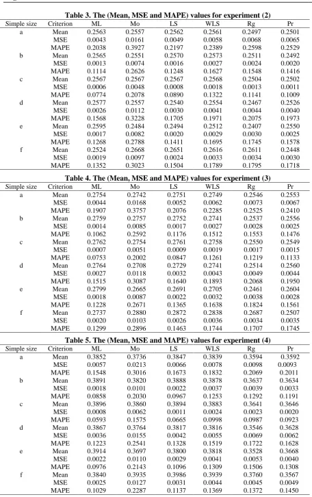
After applying the former steps of ( R ) for sample size (n1,n2,m1,m2) =a,b,c,d,e and f where

a=(15,15,15,15),b=(50,50,50,50),c=(100,100,100,10 0),d=(50,15,15,100),e=(15,100,50,100) and f=(100,50,15,50) respectively Table values (1) in

Tables (2), (3), (4), (5), (6), (7)

Table 2.The (Mean, MSE and MAPE) values for experiment (1)

Simple size Criterion ML Mo LS WLS Rg Pr

a Mean 0.2658 0.2650 0.2656 0.2655 0.2517 0.2523

MSE 0.0042 0.0213 0.0050 0.0060 0.0070 0.0064

MAPE 0.1944 0.4385 0.2116 0.2329 0.2555 0.2437

b Mean 0.2661 0.2644 0.2658 0.2655 0.2515 0.2521

MSE 0.0013 0.0122 0.0016 0.0027 0.0026 0.0022

MAPE 0.1092 0.3277 0.1220 0.1573 0.1554 0.1427

c Mean 0.2664 0.2657 0.2662 0.2656 0.2517 0.2522

MSE 0.0007 0.0091 0.0008 0.0019 0.0015 0.0012

MAPE 0.0772 0.2785 0.0871 0.1297 0.1167 0.1058

d Mean 0.2680 0.2576 0.2644 0.2652 0.2493 0.2539

MSE 0.0027 0.0161 0.0031 0.0042 0.0046 0.0043

MAPE 0.1556 0.3786 0.1680 0.1944 0.2073 0.1978

e Mean 0.2683 0.2487 0.2590 0.2616 0.2437 0.2549

MSE 0.0017 0.0129 0.0021 0.0031 0.0034 0.0027

MAPE 0.1249 0.3403 0.1390 0.1683 0.1776 0.1575

f Mean 0.2639 0.2862 0.2770 0.2730 0.2651 0.2480

MSE 0.0019 0.0153 0.0025 0.0034 0.0033 0.0032

MAPE 0.1323 0.3694 0.1486 0.1747 0.1718 0.1714

Table 3. The (Mean, MSE and MAPE) values for experiment (2)

Simple size Criterion ML Mo LS WLS Rg Pr

a Mean 0.2563 0.2557 0.2562 0.2561 0.2497 0.2501

MSE 0.0043 0.0161 0.0049 0.0058 0.0068 0.0065

MAPE 0.2038 0.3927 0.2197 0.2389 0.2598 0.2529

b Mean 0.2565 0.2551 0.2570 0.2573 0.2511 0.2492

MSE 0.0013 0.0074 0.0016 0.0027 0.0024 0.0020

MAPE 0.1114 0.2626 0.1248 0.1627 0.1548 0.1416

c Mean 0.2567 0.2567 0.2567 0.2568 0.2504 0.2502

MSE 0.0006 0.0048 0.0008 0.0018 0.0013 0.0011

MAPE 0.0774 0.2078 0.0890 0.1322 0.1141 0.1009

d Mean 0.2577 0.2557 0.2540 0.2554 0.2467 0.2526

MSE 0.0026 0.0112 0.0030 0.0041 0.0044 0.0040

MAPE 0.1568 0.3228 0.1705 0.1971 0.2075 0.1973

e Mean 0.2595 0.2484 0.2494 0.2512 0.2407 0.2550

MSE 0.0017 0.0082 0.0020 0.0029 0.0030 0.0025

MAPE 0.1268 0.2788 0.1411 0.1695 0.1745 0.1578

f Mean 0.2524 0.2668 0.2651 0.2616 0.2611 0.2448

MSE 0.0019 0.0097 0.0024 0.0033 0.0034 0.0030

MAPE 0.1352 0.3023 0.1504 0.1789 0.1795 0.1718

Table 4. The (Mean, MSE and MAPE) values for experiment (3)

Simple size Criterion ML Mo LS WLS Rg Pr

a Mean 0.2754 0.2742 0.2751 0.2749 0.2546 0.2553

MSE 0.0044 0.0168 0.0052 0.0062 0.0073 0.0067

MAPE 0.1907 0.3757 0.2076 0.2285 0.2525 0.2410

b Mean 0.2759 0.2757 0.2752 0.2741 0.2537 0.2556

MSE 0.0014 0.0085 0.0017 0.0027 0.0028 0.0025

MAPE 0.1062 0.2592 0.1176 0.1512 0.1553 0.1476

c Mean 0.2762 0.2754 0.2761 0.2758 0.2550 0.2549

MSE 0.0007 0.0051 0.0009 0.0019 0.0017 0.0015

MAPE 0.0753 0.2002 0.0847 0.1261 0.1219 0.1133

d Mean 0.2764 0.2708 0.2729 0.2741 0.2514 0.2560

MSE 0.0027 0.0118 0.0032 0.0043 0.0049 0.0044

MAPE 0.1515 0.3087 0.1640 0.1893 0.2068 0.1950

e Mean 0.2799 0.2665 0.2691 0.2705 0.2461 0.2604

MSE 0.0018 0.0087 0.0022 0.0032 0.0038 0.0028

MAPE 0.1228 0.2671 0.1365 0.1638 0.1824 0.1561

f Mean 0.2737 0.2880 0.2872 0.2838 0.2687 0.2507

MSE 0.0020 0.0103 0.0026 0.0036 0.0034 0.0035

MAPE 0.1299 0.2896 0.1463 0.1744 0.1707 0.1745

Table 5. The (Mean, MSE and MAPE) values for experiment (4)

Simple size Criterion ML Mo LS WLS Rg Pr

a Mean 0.3852 0.3736 0.3847 0.3839 0.3594 0.3592

MSE 0.0057 0.0213 0.0066 0.0078 0.0098 0.0093

MAPE 0.1548 0.3016 0.1673 0.1832 0.2069 0.2011

b Mean 0.3891 0.3820 0.3888 0.3878 0.3637 0.3634

MSE 0.0018 0.0101 0.0022 0.0037 0.0039 0.0033

MAPE 0.0858 0.2030 0.0967 0.1253 0.1292 0.1191

c Mean 0.3896 0.3860 0.3894 0.3883 0.3641 0.3646

MSE 0.0008 0.0062 0.0011 0.0024 0.0023 0.0020

MAPE 0.0593 0.1575 0.0665 0.0998 0.0987 0.0923

d Mean 0.3867 0.3764 0.3817 0.3816 0.3546 0.3628

MSE 0.0036 0.0155 0.0042 0.0055 0.0069 0.0062

MAPE 0.1223 0.2541 0.1328 0.1519 0.1722 0.1628

e Mean 0.3914 0.3697 0.3800 0.3818 0.3528 0.3668

MSE 0.0022 0.0110 0.0029 0.0041 0.0053 0.0040

MAPE 0.0976 0.2143 0.1096 0.1309 0.1506 0.1308

f Mean 0.3840 0.3935 0.3986 0.3939 0.3760 0.3567

MSE 0.0025 0.0127 0.0031 0.0044 0.0045 0.0049

Table 6. The (Mean, MSE and MAPE) values for experiment (5)

Simple size Criterion ML Mo LS WLS Rg Pr

a Mean 0.4463 0.4270 0.4462 0.4454 0.4006 0.3982

MSE 0.0061 0.0236 0.0071 0.0085 0.0121 0.0115

MAPE 0.1382 0.2712 0.1497 0.1636 0.1962 0.1908

b Mean 0.4525 0.4448 0.4515 0.4495 0.4043 0.4061

MSE 0.0019 0.0113 0.0024 0.0039 0.0058 0.0051

MAPE 0.0767 0.1831 0.0851 0.1095 0.1368 0.1298

c Mean 0.4535 0.4473 0.4532 0.4516 0.4063 0.4065

MSE 0.0009 0.0069 0.0011 0.0025 0.0040 0.0037

MAPE 0.0534 0.1407 0.0591 0.0877 0.1164 0.1134

d Mean 0.4506 0.4323 0.4459 0.4458 0.3984 0.4035

MSE 0.0037 0.0169 0.0045 0.0059 0.0090 0.0078

MAPE 0.1074 0.2248 0.1179 0.1351 0.1698 0.1584

e Mean 0.4545 0.4323 0.4419 0.4431 0.3930 0.4095

MSE 0.0025 0.0127 0.0034 0.0048 0.0081 0.0055

MAPE 0.0878 0.1966 0.1020 0.1220 0.1622 0.1331

f Mean 0.4484 0.4536 0.4632 0.4577 0.4188 0.3989

MSE 0.0026 0.0138 0.0031 0.0044 0.0054 0.0069

MAPE 0.0899 0.2031 0.0983 0.1172 0.1295 0.1491

Table 7. The (Mean, MSE and MAPE) values for experiment (6)

Simple size Criterion ML Mo LS WLS Rg Pr

a Mean 0.2296 0.2310 0.2296 0.2299 0.2034 0.2030

MSE 0.0039 0.0152 0.0045 0.0054 0.0057 0.0055

MAPE 0.2187 0.4285 0.2346 0.2565 0.2732 0.2684

b Mean 0.2278 0.2304 0.2279 0.2283 0.2007 0.2009

MSE 0.0011 0.0069 0.0014 0.0024 0.0025 0.0021

MAPE 0.1169 0.2843 0.1318 0.1732 0.1796 0.1685

c Mean 0.2281 0.2289 0.2282 0.2284 0.2008 0.2004

MSE 0.0006 0.0045 0.0007 0.0017 0.0016 0.0015

MAPE 0.0838 0.2249 0.0953 0.1425 0.1478 0.1420

d Mean 0.2296 0.2260 0.2263 0.2278 0.1990 0.2026

MSE 0.0024 0.0101 0.0027 0.0036 0.0039 0.0035

MAPE 0.1712 0.3458 0.1826 0.2093 0.2261 0.2153

e Mean 0.2311 0.2206 0.2220 0.2244 0.1940 0.2047

MSE 0.0015 0.0074 0.0018 0.0027 0.0032 0.0024

MAPE 0.1380 0.2984 0.1525 0.1860 0.2073 0.1780

f Mean 0.2242 0.2409 0.2366 0.2335 0.2110 0.1961

MSE 0.0016 0.0086 0.0022 0.0031 0.0028 0.0030

MAPE 0.1423 0.3184 0.1626 0.1935 0.1883 0.1972

Conclusions:

These conclusions are according to the results of simulation:

A. We conclude from table (1) the following: 1- Reliability of model decreases with the increasing values of 𝜎 .

2- Reliability of model increases with the increasing values of 𝜌1 and 𝜌2 .

3- Reliability of model decreases with the increasing values of 𝜃1 and 𝜃2 .

4- Reliability of model increases with decreasing values of ( _mk ) .

B. The best estimation method for Reliability of MSE and MAPE:

Values of parameters and samples sizes Best

method

For (n1, n2, m1, m2) =

(15,15,15,15), (50,50,50,50), (100,100,100,100),

(50,15,15,100), (15,100,50,100) and (100,50,15,50)

when

(α, β1, β2, μ1, μ2) =

(1.5,1.5,1.5,1.5,1.5), (2,1.5,1.5,1.5,1.5)

for k = 1.8, m = 0.3

(α, β1, β2, μ1, μ2) =

(2,1.5,1.5,1.5,1.5), (, 2,3,3,2,2) for k = 1.5, m = 0.5

(α, β1, β2, μ1, μ2) = (2,3,3,2,2), (2,2,2,3,3)

for k = 1.25, m = 0.8

ML

References:

1. Ozler B S, Gurler S. On the Reliability of k-OUT-OF-n: F system with Exchangeable components in the stress-strength setup TWMS Journal of Applied and Engineering Mathematics. 2012; 2 (1): 109-115. 2. Gogoi J, Borah M. Inference on Reliability for

Cascade Model. . Journal of Informatics and Mathematical Science s. 2012; 4 (1): 77-83.

3. Sandhya K, Umamaheswari T S. Reliability of a multi component stress strength model with standby

system using mixture of two exponential

distribution. Journal of Reliability and Statistical Studies. 2013; 6 (2) : 105-113 .

4. Umamaheswari T S, Swathi N . Cascade reliability

for generalized exponential distribution.

International IJCER. 2013; 3 (1): 132-136

5. Singh D. Measuring Reliability of n-cascade system under random stress attention. IJSER . 2013; 4 (12):1400-1404.

6. Reddy D . Cascade and system Reliability for exponential distributions. DJ Journal of Engineering and Applied Mathematics. 2016 ; 2 (2) :1-8 .

7. Devi M T, Umamaheswari T S, Swathi N. Cascade system Reliability with stress and strength follow Lindley distribution. IJERT. 2016 September; 5 (9):708-714.

8. Mutkekar R R, Munoli S B. Estimation of Reliability for stress-strength cascade model. OJS. 2016; 6: 873-881

9. Karam N S, Husieen H. Frechet Cascade Stress-Strength System Reliability. Mathematical Theory and Modeling. 2017; 7 (11):12-19.

10. Karam N S, Khaleel A H. Weibull reliability estimation for (2+1) cascade model. IJAMS. 2018; 6 (1):19-23.

11. Alqallaf F, Ghitany M E, Agostinelli C. Weighted Exponential Distribution Different Methods of Estimations. AMIS. 2015; 9 (3):1167-1173.

12. Guney Y, Arslan O .Robust parameter estimation for the Marshall-Olkin extended BURR XII distribution. Communications de la Faculté des Sciences de l University Ankara Séries A1. 2017; 66 (2) :141-161.

ريدقت

لا ةلاد

( داكساك جذومنل ةيلوعم

2

+

1

)

ليلخ نوراه دمحأ

مرك حابص ىدن

1

قارعلا ,راق يذ ,رموس ةعماج ,داصتقلااو ةرادلاا ةيلك ,ءاصحلاا مسق

2

,تايضايرلا مسق ةيبرتلا ةيلك

, ةيرصنتسملا ةعماجلا دادغب ,

, قارعلا

: ةصلاخلا

( داكسك جذومن ةيلوعم ثحبلا اذه شقاني 1

+ 2 داة جلااو ةةناتملا موةكت امدةند جذوةمنلا ةةيلوعم داجيا مت . لبيو سوكعم عيزوتل ) اةم ل

ةرغةصلا تاةعبرملا , موزعلا , مظدلاا ماكملاا( ريدقت قرط تس . ةمولعم لكشلا ةملعمو ةمولعم ريغ سايقلا ةملعم ثيح لبيو سوكعم عيزوت ةساوب ةة لتدملا فتةسلا قرةسلا قيةب ةةنراقملا . ةةيلوعملا تاريدةقت داةجيي تمددتةسا ) ةيؤملا بترلا و رادحنلاا , ةحجرملا ةرغصلا تاعبرملا ةس

بلاتام ةسساوب ةاكاحملا ةسارد 2016

ثةيح, يةلسملا لبةسنلا أةسدلا طةسوتم رايعم و أسدلا عبرم طسوتم امه قييئاصحا قيرايعم ماددتساب ,

. مظدلاا ماكملاا ردقم وه ةتسلا تاردقملا قيب ريدقت لضفا ما دجو

ةيحاتفملا تاملكلا :

د ,سايقلا ةملعم ,ةرغصلا تاعبرملا ,قيهوتلا لما ةناتم ,ةاكاحملا