Atmos. Meas. Tech., 6, 937–948, 2013 www.atmos-meas-tech.net/6/937/2013/ doi:10.5194/amt-6-937-2013
© Author(s) 2013. CC Attribution 3.0 License.
EGU Journal Logos (RGB)
Advances in
Geosciences
Open Access
Natural Hazards
and Earth System
Sciences
Open Access
Annales
Geophysicae
Open Access
Nonlinear Processes
in Geophysics
Open Access
Atmospheric
Chemistry
and Physics
Open Access
Atmospheric
Chemistry
and Physics
Open Access
Discussions
Atmospheric
Measurement
Techniques
Open Access
Atmospheric
Measurement
Techniques
Open Access
Discussions
Biogeosciences
Open Access Open Access
Biogeosciences
Discussions
Climate
of the Past
Open Access Open Access
Climate
of the Past
Discussions
Earth System
Dynamics
Open Access Open Access
Earth System
Dynamics
Discussions
Geoscientific
Instrumentation
Methods and
Data Systems
Open Access
Geoscientific
Instrumentation
Methods and
Data Systems
Open Access
Discussions
Geoscientific
Model Development
Open Access Open Access
Geoscientific
Model Development
Discussions
Hydrology and
Earth System
Sciences
Open Access
Hydrology and
Earth System
Sciences
Open Access
Discussions
Ocean Science
Open Access Open Access
Ocean Science
Discussions
Solid Earth
Open Access Open Access
Solid Earth
DiscussionsThe Cryosphere
Open Access Open Access
The Cryosphere
Discussions
Natural Hazards
and Earth System
Sciences
Open Access
Discussions
Climatologies from satellite measurements: the impact of orbital
sampling on the standard error of the mean
M. Toohey1and T. von Clarmann2
1GEOMAR Helmholtz-Centre for Ocean Research Kiel, Kiel, Germany
2Karlsruhe Institute of Technology, Institute for Meteorology and Climate Research, Karlsruhe, Germany Correspondence to: M. Toohey ([email protected])
Received: 31 October 2012 – Published in Atmos. Meas. Tech. Discuss.: 9 November 2012 Revised: 19 February 2013 – Accepted: 10 March 2013 – Published: 10 April 2013
Abstract. Climatologies of atmospheric observations are
of-ten produced by binning measurements according to latitude and calculating zonal means. The uncertainty in these cli-matological means is characterised by the standard error of the mean (SEM). However, the usual estimator of the SEM, i.e., the sample standard deviation divided by the square root of the sample size, holds only for uncorrelated ran-domly sampled measurements. Measurements of the atmo-spheric state along a satellite orbit cannot always be con-sidered as independent because (a) the time-space interval between two nearest observations is often smaller than the typical scale of variations in the atmospheric state, and (b) the regular time-space sampling pattern of a satellite instru-ment strongly deviates from random sampling. We have de-veloped a numerical experiment where global chemical fields from a chemistry climate model are sampled according to real sampling patterns of satellite-borne instruments. As case studies, the model fields are sampled using sampling patterns of the Michelson Interferometer for Passive Atmospheric Sounding (MIPAS) and Atmospheric Chemistry Experiment Fourier-Transform Spectrometer (ACE-FTS) satellite instru-ments. Through an iterative subsampling technique, and by incorporating information on the random errors of the MI-PAS and ACE-FTS measurements, we produce empirical es-timates of the standard error of monthly mean zonal mean model O3in 5◦latitude bins. We find that generally the
clas-sic SEM estimator is a conservative estimate of the SEM, i.e., the empirical SEM is often less than or approximately equal to the classic estimate. Exceptions occur only when natural variability is larger than the random measurement error, and specifically in instances where the zonal sampling distribu-tion shows non-uniformity with a similar zonal structure as
variations in the sampled field, leading to maximum sensitiv-ity to arbitrary phase shifts between the sample distribution and sampled field. The occurrence of such instances is thus very sensitive to slight changes in the sampling distribution, and to the variations in the measured field. This study high-lights the need for caution in the interpretation of the oft-used classically computed SEM, and outlines a relatively simple methodology that can be used to assess one component of the uncertainty in monthly mean zonal mean climatologies pro-duced from measurements from satellite-borne instruments.
1 Introduction
Atmospheric observations are often averaged within time-space intervals, such as calendar months and latitude bands, producing so-called “climatologies” (e.g., Grooß and Russell III, 2005; Hegglin and Tegtmeier, 2011; von Clarmann et al., 2012). While the motives behind the con-struction of such climatologies can be simply pragmatic – for instance to simplify comparison with similarly averaged model fields – averaging does have the advantageous effect of reducing the impact of random variations present in indi-vidual measurements due to measurement errors and natural variability. The standard error of the mean (SEM) is a statis-tical quantity which quantifies the random error in the calcu-lated mean value.
SEM estimator is given by the standard deviation of the sam-ple divided by the square root of the samsam-ple size, however, this estimator is only valid when the measurements are un-correlated. Consideration of correlations of measured data is a standard in various applications of statistical estimators inferred from atmospheric measurements, e.g., Jones et al. (1997) consider inter-site correlations in the estimation of global mean temperatures; Weatherhead et al. (1998) present a scheme to consider autocorrelations in estimating uncer-tainties in trends; and von Clarmann et al. (2010) propose a generic approach to consider arbitrary correlations in trend estimation. For the SEM, one of the most fundamental esti-mators of a finite sample of atmospheric data, little literature is available.
Correlations in atmospheric measurement sets depend upon the underlying time-space correlations of the atmo-sphere, and the time-space sampling patterns of the measure-ments themselves. Observational datasets from satellite in-struments have distinct sampling patterns which depend on the orbit and measurement technique of the instrument. Dif-ferent sampling patterns can lead to differences in the means of two datasets: in this case, the difference is referred to as a sampling bias. For example, Aghedo et al. (2011) have ex-amined the role of sampling in biasing monthly mean val-ues of satellite-based measurements of tropospheric chemi-cal species and temperature. However, the potential impact that sampling may have on the SEM of atmospheric clima-tologies has not, to our knowledge, been formally addressed. The goals of the present study are (1) to raise awareness of the potential impact of sampling on the SEM of clima-tologies built from satellite-based atmospheric measurement sets, (2) to develop a strategy for estimating the magnitude of its impact, and finally (3) to estimate the impact that sam-pling considerations have on the SEM for some sample cases. In order to assess the impact of time-space sampling patterns on the SEM, we present a numerical recipe which makes use of model fields from a coupled chemistry climate model. As-suming that the model accurately reproduces, in a statistical sense, the correlations of the true atmosphere on scales larger than the horizontal footprint of the satellite measurements, results from this experiment can be used to draw some gen-eral statements about the quality of the SEM estimates usu-ally produced from measurements.
2 Theory and methodology
Given a set ofN measurementsxn, the sample meanx and
sample standard deviationσˆxare calculated as
¯
x= PN
n=1xn
N (1)
and
ˆ
σx= s
PN
n=1(xi− ¯x)2
(N−1) (2)
respectively. The sample mean is an estimate of the pop-ulation mean, while the sample standard deviation charac-terises the scatter of the measured data and, thus, includes both the natural variability within the population and the measurement error. The sample mean is intentionally cal-culated without consideration of any predicted measurement error for weighting purposes, since measurement errors can be a function of geolocation and, thus, could bias the mean: e.g., measurement errors of gases measured by infrared emis-sion are usually smaller when the atmosphere is warmer, and inverse weighting of the measurements by the measurement error variance would bias the sample mean, so that it is more representative for the warmer parts of the atmosphere.
Each single measurement differs from the sample mean by some amount due to natural variability and measurement er-ror. Treating each such deviation as an “error”, and the sam-ple standard deviation as an estimate of the average “error”, the calculation of the SEM follows directly from generalised Gaussian error propagation:
SEM2= 1
N, . . . ,
1
N
ˆ
σx2, . . . , r1,Nσˆx2 ..
. . .. , ... rN,1σˆx2, . . . , σˆx2
1 N .. . 1 N
(3)
= ˆσx2
1+(N−1)r¯
N
, (4)
whereri,j is the correlation between measurementsxi and xj, and r is the average correlation coefficient between the
measurements of the sample (cf. Jones et al., 1997). Defining
k=p1+(N−1)r, (5)
the SEM can be written as SEM=√σxˆ
Nk. (6)
With r=0, i.e., independent uncorrelated measurements (both in terms of measurement error and natural variabil-ity),k=1 and the expression for the SEM simplifies to its common estimator σˆx/
√
N. When the average correlation between measurements is positive, k >1 and the SEM is greater thanσˆx/
√
N, i.e., the usual estimator which assumes independent measurements can be seen to underestimate the true SEM. Likewise, when the average correlation between measurements is negative (but not less than−1/(N−1)), 0< k <1 and the usual estimator,σx/ˆ
√
N, is an overesti-mate of the true SEM.
Since the variance of the measurements is due to both nat-ural variability and to measurement noise, the SEM reflects both sources of variance. Assuming that measurement indi-vidual error (i) of any individual measurement (xi) is
un-correlated with the true atmospheric state (τi), the variance
of any measurement setσˆx2is equal to the sum of the vari-ances of the truth and the measurement error:
ˆ
Under these standard assumptions, the SEM can be similarly decomposed into components reflecting uncertainty in the mean due to natural and measurement error variability:
SEM2=SEM2τ+SEM2. (8)
In situations where SEM2SEM2τ, i.e., where retrievals have large random errors or where the natural variability is small, the SEM reflects the uncertainty in the mean due to the random measurement error. Random measurement errors are by definition uncorrelated, therefore, the mean correlations between measurements should be negligible and the classic SEM estimator is valid in this case. In the other limiting case, where SEM2τSEM2, correlations between measurements are impacted by the patterns of variability within the atmo-sphere, leading to the possibility that correlations between measurements affect the SEM.
In this paper, we indirectly assess the role of the mean correlation coefficientr between measurements, for exam-ple satellite-borne instrument sampling patterns. We do so by producing an empirical estimate of the SEM. Here we take advantage of the fact that the SEM can be defined as the standard deviation of all possible sample means (of a given size) drawn from the population. Firstly, we subsam-ple model fields based on the sampling pattern of a satellite instrument. Leaving aside (for the moment) measurement er-ror, each sample of the model data can be thought of as a true value (τi) for the location of the sample. Sample means for each latitude bin are calculated from the subsampled model data for this sampling pattern. Then, we produce an “equiva-lent” sampling pattern, which reproduces the most important features of the sampling (latitude and local solar time), but is randomly shifted in longitude (and universal time such that local solar time is held constant). Each such equivalent sam-pling pattern can be thought of as resulting from a satellite instrument which has the exact same orbit as the original, ex-cept with a different position along the orbit at any point in time. Performing the equivalent sampling a number of times (J), we produce an ensemble of equally probable sample means for each bin (τj). The expected value of the sample
meanhτjiis taken to be the ensemble mean of the sample
means, the error of each ensemble mean is, thus,τj− hτji
and the SEM is: SEM2τ =
J
X
j=1
(τ¯j− hτji)2
J−1 . (9)
Another option would be to replace the expectation value hτji in Eq. (9) by the true average of all modelled values
in the latitude/time bin under consideration. In this case, the resulting standard error of the mean would also include any potential sampling bias, while our analysis aims at the as-sessment of the random error.
Since correlations between the random errors of measure-ments should be negligible, the random error component of the SEM can be easily calculated as
SEM2=σ
2
N, (10)
thus, in order to estimate the total SEM for any instrument dataset, one requires an estimate of the SEM due to sam-pling of the atmosphere’s natural variability (through the re-sampling exercise and Eq. (9) and knowledge of the random uncertainty in the measurements, given as the error variance
σ2.
The magnitude of the impact of correlations on the SEM will be quantified by computing values ofkthrough Eq. (6), by taking the ratio of the empirical SEM and a classic SEM estimator. Substituting Eqs. (7), (8) and (10) into Eq. (6), we can estimatekbased on quantities described above as:
k2=SEM
2
τ+σ2/N σ2
τ/N+σ2/N
. (11)
3 Case Studies
3.1 Data
3.1.1 MIPAS sampling
The Michelson Interferometer for Passive Atmospheric Sounding (MIPAS) was a mid-infrared Fourier transform limb emission spectrometer designed and operated for mea-surement of atmospheric trace species from space (Fischer et al., 2008). MIPAS passed the equator in a southerly di-rection at 10:00 local time 14.3 times a day, observing the atmosphere during day and night with global coverage from pole to pole.
Two different sampling patterns from the MIPAS mission are used here. From July 2002 to March 2004, MIPAS oper-ated at full spectral resolution, and recorded profiles of limb spectra every 90 s, corresponding to an along-track sampling of approximately 500 km, providing about 1000 vertical pro-files per day in its standard observation mode. The latitudes of each MIPAS profile spectra were nominally fixed, i.e., for the majority of orbits, profiles were repeatedly measured at specific latitudes. The sampling pattern associated with this period of high spectral resolution MIPAS measurements is referred to as MIPAS-HR.
refer to high and low spectral resolution, respectively, which correspond in contrast to low and high time-space sample resolution, respectively.)
We have taken actual measurement locations for MI-PAS measurements from 13 January–17 February 2003 and 22 December 2008–26 January 2009 as example sample pat-terns for MIPAS-HR and MIPAS-LR periods, respectively. Since there are no drastic differences between the month-to-month sampling patterns of MIPAS (aside from the change between the HR and LR sampling patterns), the sampling patterns from these time periods have been used to define the example sampling patterns for all calendar months for the two periods. It should be noted that since these are actual measurement locations, there are some deviations from the nominal sampling patterns, e.g., sample locations removed because of poor data quality or retrieval problems.
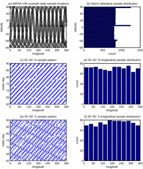
Sampling characteristics for the MIPAS sampling patterns are shown in Figs. 1 and 2. Example daily sample loca-tions for MIPAS-HR (Fig. 1a) span 87.10◦S to 89.25◦N latitude, with approximately 1000 sample locations per day. Over a full month of sampling, around 800 samples are col-lected within 5◦ latitude bins (Fig. 1b). Since the latitudi-nal spacing of consecutive measurements is approximately 5◦(median difference of 4.77◦), consecutive measurements are generally not grouped into the same latitude bin (ex-ceptions occurring within the 5–10◦N and 85–90◦N bins), therefore, consecutive measurements within one latitude bin occur during ascending and descending portions of a single orbit and, as a result, the longitude spacing between consec-utive measurements within one latitude bin is approximately 180◦longitude (median difference of 177◦). Taking an
exam-ple latitude bin, 55–60◦N, Fig. 1c shows the time (decimal
Julian day) versus longitude sampling pattern, which shows remarkable uniformity. A histogram of sample count per 30◦ longitude bin for the 55–60◦N latitude bin shows a uniform distribution of longitudinal sampling (Fig. 1d), with between 60 and 70 samples per 30◦longitude bin. A similar unifor-mity of sampling pattern is found in the example Southern Hemisphere (SH) latitude bin of 55–60◦S (Fig. 1e, f).
For MIPAS-LR sampling, samples are more closely spaced in time and space, and no longer fixed to certain lat-itudes. The number of monthly samples within 5◦ latitude bins is around 1000 (Fig. 2b), with some variation from bin to bin due to the more random nature of the latitudi-nal sampling. Since the time-space distance between samples is less than for the MIPAS-HR sampling case (3.6◦latitude
median difference between consecutive samples), consecu-tive measurements from the MIPAS orbit are occasionally binned within a single 5◦latitude bin. For example, approx-imately 1/4 of samples within the 55–60◦N latitude bin are “double samples”, i.e., two samples with small differences in time and space between them. In some cases, double sam-ples within a latitude bin occur preferentially within certain longitude ranges, leading to non-uniformity in the monthly zonal sample distribution. This is the case, for example, in
0 60 120 180 240 300 360 −90
−60 −30 0 30 60 90
longitude
latitude
(a) MIPAS−HR example daily sample locations
0 500 1000 1500
−90 −60 −30 0 30 60 90
latitude
count
(b) March latitudinal sample distribution
0 60 120 180 240 300 360 60
65 70 75 80 85 90
longitude
Julian day
(c) 55−60° N sample pattern
0 60 120 180 240 300 360 0
20 40 60 80
(d) 55−60° N longitudinal sample distribution
longitude
count
0 60 120 180 240 300 360 60
65 70 75 80 85 90
longitude
Julian day
(e) 55−60° S sample pattern
0 60 120 180 240 300 360 0
20 40 60 80
(f) 55−60° S longitudinal sample distribution
longitude
count
Fig. 1. MIPAS-HR March sampling, approximating MIPAS sam-pling over the time interval July 2002 to March 2004. (a) Example daily sampling spatial pattern, (b) monthly sample counts per 5◦ latitude bin, (c) time, longitude pattern of samples and (d) zonal sample distribution for the 55–60◦N latitude bin, (e) time, longi-tude pattern of samples and (f) zonal sample distribution for the 55–60◦S latitude bin.
the 55–60◦S bin (Fig. 2e, f), with a notable excess of sam-ples in the Eastern Hemisphere (0–180◦longitude). Within the 55–60◦N bin, however, the double samples are more ran-domly (and uniformly) distributed (Fig. 2c), and the resulting zonal sample distribution (Fig. 2d) is of similar uniformity as that of MIPAS-HR.
3.1.2 ACE-FTS sampling
0 60 120 180 240 300 360 −90
−60 −30 0 30 60 90
longitude
latitude
(a) MIPAS−LR example daily sample locations
0 500 1000 1500
−90 −60 −30 0 30 60 90
latitude
count
(b) March latitudinal sample distribution
0 60 120 180 240 300 360 60
65 70 75 80 85 90
longitude
Julian day
(c) 55−60° N sample pattern
0 60 120 180 240 300 360 0
20 40 60 80 100
(d) 55−60° N longitudinal sample distribution
longitude
count
0 60 120 180 240 300 360 60
65 70 75 80 85 90
longitude
Julian day
(e) 55−60° S sample pattern
0 60 120 180 240 300 360 0
20 40 60 80 100 120
(f) 55−60° S longitudinal sample distribution
longitude
count
Fig. 2. MIPAS-LR March sampling, approximating MIPAS sam-pling from January 2005 until mission conclusion. (a) Example daily sampling spatial pattern, (b) monthly sample counts per 5◦ latitude bin, (c) time, longitude pattern of samples and (d) zonal sample distribution for the 55–60◦N latitude bin, (e) time, longi-tude pattern of samples and (f) zonal sample distribution for the 55–60◦S latitude bin.
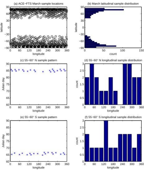
For the sampling exercise presented here, we use the ACE-FTS sampling locations from the year 2005, and examine the months March and April as example cases – March gives rea-sonable coverage of both the southern and northern mid- and high-latitudes, while April sampling covers the tropics and subtropics. Characteristics of the sample patterns for ACE-FTS in March and April are shown in Figs. 3 and 4. For March, highest sample density is found in the high latitudes, which is a product of design, the ACE mission being fo-cused on obtaining measurements during the polar winters and springs when O3destruction chemical processes are
un-derway (Bernath et al., 2005). Sample counts within 5◦ lati-tude bins for March range between∼10 to∼80 depending on latitude within this month. For the example latitude bin of 55–60◦N, ACE-FTS samples are collected over a few days
near the end of the month (Fig. 3c) while in the 55–60◦S bin,
ACE-FTS samples are collected over a few days at the begin-ning of the month (Fig. 3e). Within this time frame, the sam-ples circle the Earth in terms of longitude, and the distribu-tion of longitudes sampled is, thus, relatively uniform given such small sample size, (Fig. 3d, f), with non-uniformity occurring because of missing measurements or overlap of longitudinal sampling cycles. At latitudes higher than the
0 60 120 180 240 300 360 −90
−60 −30 0 30 60 90
longitude
latitude
(a) ACE−FTS March sample locations
0 50 100 150
−90 −60 −30 0 30 60 90
latitude
count
(b) March latitudinal sample distribution
0 60 120 180 240 300 360 60
65 70 75 80 85 90
longitude
Julian day
(c) 55−60° N sample pattern
0 60 120 180 240 300 360 0
0.5 1 1.5 2 2.5 3
(d) 55−60° N longitudinal sample distribution
longitude
count
0 60 120 180 240 300 360 60
65 70 75 80 85 90
longitude
Julian day
(e) 55−60° S sample pattern
0 60 120 180 240 300 360 0
0.5 1 1.5 2 2.5 3
(f) 55−60° S longitudinal sample distribution
longitude
count
Fig. 3. ACE-FTS sampling in March 2005. (a) Full monthly sam-pling spatial pattern, (b) monthly sample counts per 5◦latitude bin, (c) time, longitude pattern of samples and (d) zonal sample distri-bution for the 55–60◦N latitude bin, (e) time, longitude pattern of samples and (f) zonal sample distribution for the 55–60◦S latitude bin.
55–60◦ bands shown here, sampling density increases sub-stantially (Fig. 3b), and the zonal distributions become more uniform, while at lower latitudes, the opposite is true.
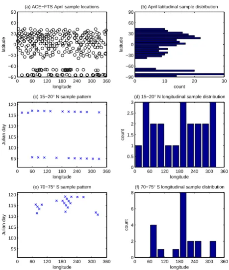
In April, the ACE-FTS sunrise and sunset sampling pat-terns cross through the tropics (Fig. 4a). Taking 15–20◦N as an example latitude bin in the tropics, we see that samples for this bin are composed of measurements at the beginning and end of the month (Fig. 4c). The longitude spacing between consecutive measurements is nominally 24.5◦, and samples are collected in this bin over∼2 days, long enough for the samples to cover the full zonal band, leading to 2 or more samples within 9 out of the 12 30◦longitude bins shown in
Fig. 4d. There are also a handful of samples within April in the SH high latitudes. Taking the example band of 70–75◦S, these samples are collected near the end of April (Fig. 4e), and are notably non-uniform in their longitudinal distribu-tion (Fig. 4f).
3.1.3 Model fields
0 60 120 180 240 300 360 −90
−60 −30 0 30 60 90
longitude
latitude
(a) ACE−FTS April sample locations
0 10 20 30
−90 −60 −30 0 30 60 90
latitude
count
(b) April latitudinal sample distribution
0 60 120 180 240 300 360 95
100 105 110 115 120
longitude
Julian day
(c) 15−20° N sample pattern
0 60 120 180 240 300 360 0
0.5 1 1.5 2 2.5 3
(d) 15−20° N longitudinal sample distribution
longitude
count
0 60 120 180 240 300 360 95
100 105 110 115 120
longitude
Julian day
(e) 70−75° S sample pattern
0 60 120 180 240 300 360 0
2 4 6 8
(f) 70−75° S longitudinal sample distribution
longitude
count
Fig. 4. ACE-FTS sampling from April 2005. (a) Full monthly sam-pling spatial pattern, (b) monthly sample counts per 5◦latitude bin, (c) time, longitude pattern of samples and (d) zonal sample distri-bution for the 15–20◦N latitude bin, (e) time, longitude pattern of samples and (f) zonal sample distribution for the 70–75◦S latitude bin.
(1997), respectively. Simulated chemical fields from a sin-gle year (1996) of the CMAM REF1 simulation described by Eyring et al. (2006) are used here. The chemical fields are available for every model gridpoint with 3.75◦by 3.75◦ resolution in intervals of 18 h.
The distributions of chemical species in the CMAM have been seen to generally compare well with observations (e.g. de Grandpr´e et al., 2000; Farahani et al., 2007; Hegglin and Shepherd, 2007; Jin et al., 2005; Jin et al., 2009; Melo et al., 2008). While this version of CMAM does not simu-late the quasi-biennial oscillation and, thus, underestimates interannual variability in the tropics, the intra-month vari-ability appears to be of realistic magnitude (see Chapter 7 of SPARC CCMVal, 2010; Toohey et al., 2010). The persis-tence (i.e., autocorrelation) of zonal mean O3 anomalies in
CMAM agrees extremely well with observations, with inter-annual anomalies established through winter and spring per-sisting with very high correlation coefficients through sum-mer until early autumn (Tegtmeier and Shepherd, 2007).
Figure 5 shows the monthly mean zonal mean O3
distribu-tion for March, as well as the monthly zonal standard devia-tion (SD) for each latitude and height. Maxima in short-term (intra-monthly) O3 variability are found generally where
mean
latitude
pressure (hPa)
−90 −60 −30 0 30 60 90 10−1
100
101
102
103
ppmv
0 5 10
standard deviation
latitude
−90 −60 −30 0 30 60 90 10−1
100
101
102
103
ppmv
0 0.5 1
Fig. 5. CMAM March O3: (left) monthly mean zonal mean O3and (right) monthly zonal standard deviation O3as function of latitude
and pressure.
spatial gradients in O3 are strong. Variability is generally
weak during summer months, therefore, examining variabil-ity around the equinoxes allows for a case when there is ap-preciable variability in both hemispheres.
3.1.4 Measurement random errors
MIPAS random error estimates for O3measurements during
the HR period are taken from the absolute values reported by Fig. 3 of Steck et al. (2007) and for the LR period from Table 7 of von Clarmann et al. (2009b). The random error es-timates for the two periods are roughly similar, with slightly larger random errors reported for the HR period. For exam-ple, absolute values of random error peak around 30 km, with values of approximately 0.35 ppmv for the HR period, and 0.3 ppmv for the LR period: percent random error between approximately 20 and 40 km altitudes are reported as 5–6 % for the HR period and 4–5 % for the LR period.
ACE-FTS random error estimates for O3are taken as the
root-mean-square of the random errors reported in ACE-FTS v2.2 O3 update dataset for the month of March 2005. This
random error profile is approximately equal to the profile re-ported for tropical retrievals shown in Fig. 6a of Toohey et al. (2010), with peak value of approximately 0.15 ppmv around 30 km, and percent values of 1–2 % between 20 and 60 km. It should be noted that the reported random errors of the ACE-FTS measurements consider only measurement noise, and not other factors (e.g., pointing uncertainty) that may also lead to random errors in the retrieved profiles.
3.2 Sampling procedure
latitude
pressure (hPa)
(a) στ N−1/2
−90 −45 0 45 90 10−1
100
101
102
103
ppmv 0 0.02 0.04
latitude (c) SEM τ
−90 −45 0 45 90 10−1
100
101
102
103
ppmv 0 0.02 0.04 latitude
(b) σε N−1/2
−90 −45 0 45 90 10−1
100
101
102
103
ppmv 0 0.02 0.04
latitude (d) k
−90 −45 0 45 90 10−1
100
101
102
103
0.5 1 1.5 2
latitude
pressure (hPa)
(e) στ N−1/2
−90 −45 0 45 90 10−1
100
101
102
103
ppmv 0 0.02 0.04
latitude (g) SEMτ
−90 −45 0 45 90 10−1
100
101
102
103
ppmv 0 0.02 0.04 latitude
(f) σε N−1/2
−90 −45 0 45 90 10−1
100
101
102
103
ppmv 0 0.02 0.04
latitude (h) k
−90 −45 0 45 90 10−1
100
101
102
103
0.5 1 1.5 2
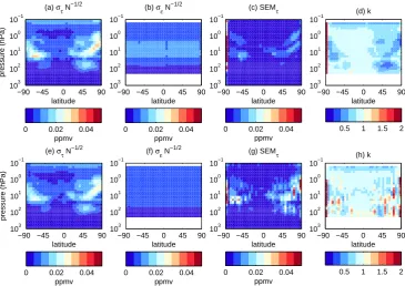
Fig. 6. Pressure latitude sections of zonal mean values ofστ/
√
N, the single-sample estimate of the natural variability component of the SEM (first column);σ/
√
N, the random measurement error component of the SEM (second column); the empirically derived SEMτ(third
column) andkas defined in text (fourth column) based on MIPAS-HR (top) and MIPAS-LR (bottom) sampling of CMAM March O3.
pattern was adjusted by producing a random numberyfrom the uniform distribution over the interval (0,1) and adding a term 360y to the vector of longitudes, and subtracting 24y
from the time vector. Twenty ensemble members were cre-ated for each sampling pattern, and used to sample the model fields.
Given the 18 h temporal resolution of the model fields used here, we expect this sampling exercise to be valid only for long-lived chemical species. Variations of O3, which has a
lifetime of days to weeks in the lower and middle strato-sphere, should be adequately described by 18 h fields except in the upper stratosphere and mesosphere where diurnal vari-ations become important. Application of the sampling exper-iment to other chemical species with shorter lifetimes would require the use of model fields with higher temporal resolu-tion.
In general, the variability of sampled atmospheric fields depends on the resolution of the sample, with many pro-cesses (gravity waves, for example) that produce variabil-ity on small scales which will have negligible impacts over larger scales. It is, therefore, important for the resolution of the sampled model fields to be similar to the resolution expected of the atmospheric measurements. In the present case, the horizontal resolution of the CMAM fields is 3.75◦, or roughly 400 km, which is comparable to the horizontal resolutions of the ACE-FTS (ca. 500 km) and MIPAS (ca. 400 km, von Clarmann et al., 2009a) measurements. For this
reason we have performed no smoothing of the model fields, although this would be necessary in the case that the model fields were of significantly finer resolution than the measure-ments. It should also be noted that in order for the present exercise to to applied to nadir-sounding instruments with fine horizontal resolution, model fields with similarly fine resolu-tion would be required.
3.3 Results
3.3.1 MIPAS
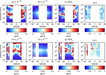
Figure 6a–d shows results of the resampling exercise for MIPAS-HR sampling of O3over the month of March.
Fig-ure 6a shows the sample SD divided by the square root of sample size, corresponding to a single-sample estimate of SEMτ. This quantity follows the natural variability of the O3
field, with maximum values of∼0.03 ppmv in the mid- to high latitudes of the middle stratosphere, reflecting the ratio of maximum model variability (∼1 ppmv, see Fig. 5) to the square root of the sample size (∼800).
The SEM due to measurement error, σ/
√
N, is shown in Fig. 6b. This quantity is comparable in magnitude to that shown in 6a, except in regions where natural variabil-ity reaches its maximum values.
The SEMτ estimated through the ensemble resampling
technique (Fig. 6c) is notably smaller thanστ/
√
latitude
pressure (hPa)
(a) στ N−1/2
−90 −45 0 45 90 10−1
100
101
102
103
ppmv
0 0.05 0.1
latitude (c) SEM
τ
−90 −45 0 45 90 10−1
100
101
102
103
ppmv
0 0.05 0.1
latitude (b) σε N−1/2
−90 −45 0 45 90 10−1
100
101
102
103
ppmv
0 0.05 0.1
latitude (d) k
−90 −45 0 45 90 10−1
100
101
102
103
0.5 1 1.5 2
latitude
pressure (hPa)
(e) στ N−1/2
−90 −45 0 45 90 10−1
100
101
102
103
ppmv
0 0.05 0.1
latitude (g) SEMτ
−90 −45 0 45 90 10−1
100
101
102
103
ppmv
0 0.05 0.1
latitude (f) σε N−1/2
−90 −45 0 45 90 10−1
100
101
102
103
ppmv
0 0.05 0.1
latitude (h) k
−90 −45 0 45 90 10−1
100
101
102
103
0.5 1 1.5 2
Fig. 7. Pressure latitude sections of zonal mean values ofστ/
√
N, the single-sample estimate of the natural variability component of the SEM (first column);σ/
√
N, the random measurement error component of the SEM (second column); the empirically derived SEMτ(third
column) andkas defined in text (fourth column) based on ACE-FTS sampling of CMAM March (top) and April (bottom) O3.
sampling pattern of MIPAS-HR, the sample mean is appar-ently quite insensitive to shifts in the longitudinal distribu-tion. As a result,kvalues (Fig. 6d) are less than 1 throughout almost all of the stratosphere. In regions whereσ/
√
N is greater thanστ/
√
N, such as throughout most of the tropical stratosphere,k values approach 1. In regions of significant natural variability, i.e., in the mid- to high latitudes of both hemispheres,kvales are small, reflecting the difference be-tweenστ/
√
N and SEMτ. In these regions the classic SEM
estimator overestimates the true SEM given the MIPAS-HR sampling, in other words, in this case the classic SEM is a conservative estimate of the true SEM.
Figure 6e–h shows results of the resampling exercise for MIPAS-LR sampling of O3 over March. Due to its larger
sample sizes,στ/
√
N (Fig. 6e) for MIPAS-LR sampling is slightly smaller than that for MIPAS-HR. The SEM due to measurement error,σ/
√
N(Fig. 6f) is slightly smaller than its comparable quantity for the MIPAS-HR sampling due to larger sample sizes and the slightly smaller random error for the LR period retrievals. As for MIPAS-HR sampling, the SEMτ estimated through the ensemble resampling
tech-nique for MIPAS-LR sampling (Fig. 6g) is generally less thanστ/
√
N, however, the results for MIPAS-LR sampling show a closer agreement between the two quantities than for MIPAS-HR. We interpret this result as a consequence of dif-ferences in the sampling patterns of the two MIPAS periods. With sampled latitudes within each bin varying from orbit
to orbit, and the closer latitude spacing leading to occasional “double samples”, MIPAS-LR sampling is a closer approxi-mation of random sampling, therefore, it stands to reason that the SEMτ values estimated through the resampling exercise
for MIPAS-LR are in closer agreement withστ/
√
Nthan for MIPAS-HR.
For MIPAS-LR, in locations of significant natural variabil-ity there are also a handful of instances of notable local max-ima in the SEMτ field, signifying cases where the sample
mean is quite sensitive to longitudinal shifts in the sampling pattern. Such values are not reflected in the στ/
√
N field, which leads tokvalues greater than 1, with the implication that in these few cases, the classic SEM estimator, computed from any one sample set, would underestimate the true SEM.
3.3.2 ACE-FTS
Figure 7 shows results of the ensemble resampling exer-cise for ACE-FTS sampling of O3 over month of March
and April. With much lower sample sizes than for MIPAS,
στ/
√
For March sampling, the SEMτ estimated through the
en-semble resampling technique (Fig. 7c) is notably smaller thanστ/
√
N for almost all latitudes and heights. As a re-sult,kvalues (Fig. 7d) are less than one throughout much of the stratosphere. As for MIPAS-LR sampling, manykvalues are relatively close to one, with 30 % ofkvalues between 0.8 and 1.2. There also exist a few isolated instances ofkvalues greater than one, where the classic SEM estimator is seen to underestimate the SEM estimated through the resampling technique.
For April sampling, the SEM estimated through the en-semble resampling technique (Fig. 7g) is generally close in value or slightly less than the classic estimator, leading tok
values approximately equal to or less than one, with 36 % of
kvalues between 0.8 and 1.2. Instances ofk >1, where the classic SEM estimator is seen to underestimate the SEM esti-mated through the resampling technique, are more prevalent than found for March sampling, with largekvalues found in the SH high latitudes and SH subtropics.
3.4 Discussion
Ignoring variations in sampling distribution with time, the resampling exercise used to produce the results in Figs. 6 and 7 can be simplified into the following: for each latitude bin, each resampled monthly mean value can be thought of as a weighted mean of the model zonal O3 field, where the
weights are defined by the zonal distribution of the monthly sample number. Each ensemble member of the resampling exercise is then produced by randomly shifting the zonal sample distribution pattern with respect to the monthly mean O3field. Variations in the monthly mean zonal mean
sam-ple means occur based on the relationship between the zonal structures of the O3field and the sampling distribution – if
either is completely uniform, then shifts in the relative zonal structure will have no effect on the sample mean. Further-more, the degree to which the ensemble of sample means vary will depend on the similarity between the two distribu-tions: maximum variation between ensemble member means should result when the mean O3field and sample distribution
have the same zonal structure.
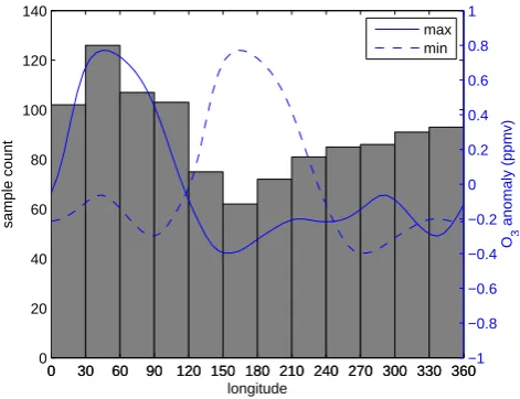
This mechanism is explored in Fig. 8 for MIPAS-LR sam-pling. In Fig. 6h, it was seen thatkvalues greater than one were found in the Northern Hemisphere (NH) mid- to high latitudes, meaning that the SEM estimated though the re-sampling exercise was found to be larger than that estimated through the classical estimator. As an example case of large
k values, we examine the 50–55◦N latitude bin at 60 hPa,
a location of a local maximum in the k values shown in Fig. 6h. Figure 8 shows a histogram of the sample distribu-tion for the MIPAS-LR sampling pattern for the 50–55◦N latitude bin separated into 30◦ longitude bins. At this lat-itude, the MIPAS-LR sampling pattern has notable zonal structure, with a maximum and minimum in sample den-sity separated by approximately 120◦. Also shown is the
0 30 60 90 120 150 180 210 240 270 300 330 360 0
20 40 60 80 100 120 140
longitude
sample count
0 30 60 90 120 150 180 210 240 270 300 330 360−1 −0.8 −0.6 −0.4 −0.2 0 0.2 0.4 0.6 0.8 1
O3
anomaly (ppmv)
max min
Fig. 8. Zonal MIPAS-LR sampling distribution for March within the 50–55◦N latitude bin (gray bars). Also shown is the monthly mean zonal O3 anomaly field at 52.4◦N, at 20 hPa. The O3field
has been shifted in longitude to produce maximum (solid) and min-imum (dashed) values of a weighted mean of the O3field using the
sample distribution as weights.
monthly mean zonal O3anomaly field for the model latitude
of 52◦at 60 hPa. The O3field has been shifted in longitude
to produce maximum (solid) and minimum (dashed) values of a weighted mean of the O3 field calculated by using the
sample distribution as weights. There is a clear correspon-dence between the structures of the sampling distribution and the O3field, and it follows that the sensitivity of the sample
mean to the phasing of the sample distribution is related to the similarity between the two distributions.
In this way, the results of the sampling exercise can be seen to be related to the correlations between the zonal structures of the sample distribution and the measured field. The results of the sampling exercise can also be interpreted in terms of correlations between individual measurements. Equation (5) shows the relationship betweenk and the mean correlation coefficient between all pairs of measurements.kvalues less than 1 imply a negative mean correlation coefficient. For measured fields with a periodic structure in longitude, sam-pled with very uniform sampling, we might expect a negative correlation since every measurement is balanced by a corre-sponding measurement on the other side of the Earth. For non-uniform sampling, e.g., when some measurements are clustered around a certain longitude, then the similarity of the O3field measured around this cluster leads to an increase
in the mean correlation, leading to mean correlation coeffi-cients approaching zero or reaching positive values, and cor-respondinglykvalues of 1 or greater, as was found for the MIPAS-LR sampling at certain locations.
Figure 9 shows a similar explanatory plot for ACE-FTS. Maximumkvalues for ACE-FTS sampling of April O3were
0 30 60 90 120 150 180 210 240 270 300 330 360 0
2 4 6 8
longitude
sample count
0 30 60 90 120 150 180 210 240 270 300 330 360 −1 −0.5 0 0.5 1
O3
anomaly (ppmv)
max min
Fig. 9. Zonal ACE-FTS sampling distribution for March within the 70–75◦S latitude bin (gray bars). Also shown is the monthly mean zonal O3 anomaly field at 74.7◦N, at 10 hPa. The O3 field has
been shifted in longitude to produce maximum (solid) and mini-mum (dashed) values of a weighted mean of the O3field using the
sample distribution as weights.
the very largekvalues are the result of a highly non-uniform sampling pattern with respect to longitude (as shown in Fig. 4), with most samples clustered within 120◦ longitude of each other. As a result of this sampling pattern, any non-uniformity in the measured O3 field will lead to variations
in the monthly mean zonal mean values produced by each realisation of the ensemble resampling, and as a result the SEM estimated by the resampling technique is large. Figure 9 shows the ACE-FTS sampling distribution for the 70–75◦S latitude band, as well as the O3anomaly field for this latitude
at 10 hPa over the days of ACE-FTS sampling of this latitude. O3anomalies show clear zonally periodic variability at this
latitude and height and, as a result, the sample mean is sensi-tive to the phase shift of the non-uniform sample distribution.
4 Conclusions
The usual way to estimate the standard error of the mean by division of the sample standard deviation by the square root of the sample size (σx/
√
N) is exact only if the elements within the sample are uncorrelated. Satellite measurement datasets, however, are not random samples because measure-ment locations are the result of factors such as the regu-lar satellite orbit and limitations of measurement frequency. Correlations between sampled points in the atmosphere may impact the measured variability such that the usual SEM es-timator is inaccurate. By subsampling model data according to the real sampling patterns of two modern satellite-borne instruments, and incorporating information of the random
errors of the instruments, this effect has been assessed for a number of test cases.
In cases where the random measurement error is larger than the natural variability, the classic SEM estimator should provide an accurate estimate of the uncertainty in the mean. However, when natural variability is larger than the random measurement error, the SEM may differ significantly from the classic estimator. Two cases with competing mechanisms have been discovered:
1. SEM< σx/
√
N: this effect is most pronounced when the sample distribution is quite uniform with respect to longitude. Since variations of stratospheric trace gases such as O3 typically follow wave like patterns along
zonal bands, within a zonal band, uniform sampling leads to negative mean correlation coefficients since each low measurement is compensated by a too-high measurement. As a result, the classical SEM es-timator, which assumes random sampling and not the highly uniform sampling of the satellite instrument overestimates the true standard error of the mean. 2. SEM> σx/
√
N: this applies particularly to cases where the zonal sampling distribution is non-uniform. If the non-uniformity of the sampling pattern is of similar zonal structure to variations in the measured field, then the measured zonal mean is sensitive to arbitrary phase shifts between the sampling pattern and the measured field. As a result, the SEM is larger than that estimated by the classic estimator. In this case, the similar zonal structure of the sampling distribution and the measured field can be understood to result in positive mean corre-lation between samples, which we suggest is an equiva-lent explanation for the fact that the classical SEM un-derestimates the true SEM.
Acknowledgements. The authors thank the instrument teams of MIPAS and ACE-FTS for providing sample patterns for use in this study, as well as Andreas I. Jonsson and Theodore G. Shepherd for providing the CMAM chemical fields. The Atmospheric Chemistry Experiment (ACE), also known as SCISAT-1, is a Canadian-led mission mainly supported by the Canadian Space Agency (CSA) and the Natural Sciences and Engineering Research Council (NSERC) of Canada. The CMAM is supported by the Canadian Foundation for Climate and Atmospheric Sciences and the CSA. M. T. acknowledges partial support through the EU project SHIVA (grant number 226224). This work was motivated by discussions within the SPARC Data initiative: the authors thank co-leaders Michaela Hegglin and Susann Tegtmeier, and all members of the SPARC DI team. Also thanks to Kaley Walker for helpful comments on a draft manuscript.
The service charges for this open access publication have been covered by a Research Centre of the Helmholtz Association.
Edited by: H. Worden
References
Aghedo, A. M., Bowman, K. W., Shindell, D. T., and Faluvegi, G.: The impact of orbital sampling, monthly averaging and vertical resolution on climate chemistry model evaluation with satellite observations, Atmos. Chem. Phys., 11, 6493–6514, doi:10.5194/acp-11-6493-2011, 2011.
Beagley, S. R., de Grandpr´e, J., Koshyk, J. N., McFarlane, N. A., and Shepherd, T. G.: Radiative-dynamical climatology of the first-generation Canadian Middle Atmosphere Model, Atmos. Ocean, 35, 293–331, doi:10.1080/07055900.1997.9649595, 1997.
Bernath, P. F., McElroy, C. T., Abrams, M. C., Boone, C. D., Butler, M., Camy-Peyret, C., Carleer, M., Clerbaux, C., Coheur, P.-F., Colin, R., DeCola, P., DeMazi`ere, M., Drummond, J. R., Du-four, D., Evans, W. F. J., Fast, H., Fussen, D., Gilbert, K., Jen-nings, D. E., Llewellyn, E. J., Lowe, R. P., Mahieu, E., Mc-Connell, J. C., McHugh, M., McLeod, S. D., Michaud, R., Mid-winter, C., Nassar, R., Nichitiu, F., Nowlan, C., Rinsland, C. P., Rochon, Y. J., Rowlands, N., Semeniuk, K., Simon, P., Skel-ton, R., Sloan, J. J., Soucy, M.-A., Strong, K., Tremblay, P., Turnbull, D., Walker, K. A., Walkty, I., Wardle, D. A., Wehrle, V., Zander, R., and Zou, J.: Atmospheric Chemistry Experiment (ACE): Mission overview, Geophys. Res. Lett., 32, L15S01, doi:10.1029/2005GL022386, 2005.
de Grandpr´e, J., Sandilands, J. W., Mcconnell, J. C., Bea-gley, S. R., Croteau, P. C., and Danilin, M. Y.: Cana-dian Middle Atmosphere Model: Preliminary results from the chemical transport module, Atmosphere–Ocean, 35, 385–431, doi:10.1080/07055900.1997.9649598, 1997.
de Grandpr´e, J., Beagley, S. R., Fomichev, V. I., Griffioen, E., Mc-Connell, J. C., Medvedev, A. S., and Shepherd, T. G.: Ozone climatology using interactive chemistry: Results from the Cana-dian Middle Atmosphere Model, J. Geophys. Res., 105, 26475– 26492, doi:10.1029/2000JD900427, 2000.
Eyring, V., Butchart, N., Waugh, D. W., Akiyoshi, H., Austin, J., Bekki, S., Bodeker, G. E., Boville, B. A., Br¨uhl, C.,
Chipper-field, M. P., Cordero, E., Dameris, M., Deushi, M., Fioletov, V. E., Frith, S. M., Garcia, R. R., Gettelman, A., Giorgetta, M. A., Grewe, V., Jourdain, L., Kinnison, D. E., Mancini, E., Manzini, E., Marchand, M., Marsh, D. R., Nagashima, T., Newman, P. A., Nielsen, J. E., Pawson, S., Pitari, G., Plummer, D. A., Rozanov, E., Schraner, M., Shepherd, T. G., Shibata, K., Stolarski, R. S., Struthers, H., Tian, W., and Yoshiki, M.: Assessment of tem-perature, trace species, and ozone in chemistry-climate model simulations of the recent past, J. Geophys. Res., 111, D22308, doi:10.1029/2006JD007327, 2006.
Farahani, E., Fast, H., Mittermeier, R. L., Makino, Y., Strong, K., McLandress, C., Shepherd, T. G., Chipperfield, M. P., Hannigan, J. W., Coffey, M. T., Mikuteit, S., Hase, F., Blu-menstock, T., and Raffalski, U.: Nitric acid measurements at Eureka obtained in winter 2001–2002 using solar and lunar Fourier transform infrared absorption spectroscopy: Compar-isons with observations at Thule and Kiruna and with results from three-dimensional models, J. Geophys. Res., 112, D01305, doi:10.1029/2006JD007096, 2007.
Fischer, H., Birk, M., Blom, C., Carli, B., Carlotti, M., von Clar-mann, T., Delbouille, L., Dudhia, A., Ehhalt, D., EndeClar-mann, M., Flaud, J. M., Gessner, R., Kleinert, A., Koopman, R., Langen, J., L´opez-Puertas, M., Mosner, P., Nett, H., Oelhaf, H., Perron, G., Remedios, J., Ridolfi, M., Stiller, G., and Zander, R.: MIPAS: an instrument for atmospheric and climate research, Atmos. Chem. Phys., 8, 2151–2188, doi:10.5194/acp-8-2151-2008, 2008. Grooß, J.-U. and Russell III, J. M.: Technical note: A stratospheric
climatology for O3, H2O, CH4, NOx, HCl and HF derived from
HALOE measurements, Atmos. Chem. Phys., 5, 2797–2807, doi:10.5194/acp-5-2797-2005, 2005.
Hegglin, M. I. and Shepherd, T. G.: O3-N2O correlations from the
Atmospheric Chemistry Experiment: Revisiting a diagnostic of transport and chemistry in the stratosphere, J. Geophys. Res., 112, 19301, doi:10.1029/2006JD008281, 2007.
Hegglin, M. I. and Tegtmeier, S.: The SPARC Data Initia-tive, SPARC Newsletter, 36, 22–23, available at: http: //www.sparc-climate.org/fileadmin/customer/6 Publications/ Newsletter PDF/36 SPARCnewsletter Jan2011.pdf (last access: 8 April 2013), 2011.
Jin, J. J., Semeniuk, K., Jonsson, A. I., Beagley, S. R., McConnell, J. C., Boone, C. D., Walker, K. A., Bernath, P. F., Rinsland, C. P., Dupuy, E., Ricaud, P., De La No¨e, J., Urban, J., and Murtagh, D.: Co-located ACE-FTS and Odin/SMR stratospheric-mesospheric CO 2004 measurements and comparison with a GCM, Geophys. Res. Lett., 32, L15S03, doi:10.1029/2005GL022433, 2005. Jin, J. J., Semeniuk, K., Beagley, S. R., Fomichev, V. I., Jonsson,
A. I., McConnell, J. C., Urban, J., Murtagh, D., Manney, G. L., Boone, C. D., Bernath, P. F., Walker, K. A., Barret, B., Ricaud, P., and Dupuy, E.: Comparison of CMAM simulations of carbon monoxide (CO), nitrous oxide (N2O), and methane (CH4) with
observations from Odin/SMR, ACE-FTS, and Aura/MLS, At-mos. Chem. Phys., 9, 3233–3252, doi:10.5194/acp-9-3233-2009, 2009.
Jones, P. D., Osborn, T. J., and Briffa, K. R.: Estimat-ing sampling errors in large-scale temperature aver-ages, J. Climate, 10, 2548–2568, doi:10.1175/1520-0442(1997)010¡2548:ESEILS¿2.0.CO;2, 1997.
F. J., Olson, J. R., Semeniuk, K., Shepherd, T. G., Strong, K., Tarasick, D., and Williams-Rioux, B. J.: Summertime strato-spheric processes at northern mid-latitudes: comparisons be-tween MANTRA balloon measurements and the Canadian Mid-dle Atmosphere Model, Atmos. Chem. Phys., 8, 2057–2071, doi:10.5194/acp-8-2057-2008, 2008.
SPARC CCMVal: SPARC Report on the Evaluation of Chemistry-Climate Models, edited by: Eyring, V., Shepherd, T. G., and Waugh, D. W., SPARC Report No. 5, WCRP-132, WMO/TD-No. 1526, available at: http://www.sparc-climate. org/publications/sparc-reports/sparc-report-no5/ (last access: 8 April 2013), 2010.
Steck, T., von Clarmann, T., Fischer, H., Funke, B., Glatthor, N., Grabowski, U., H¨opfner, M., Kellmann, S., Kiefer, M., Linden, A., Milz, M., Stiller, G. P., Wang, D. Y., Allaart, M., Blumen-stock, Th., von der Gathen, P., Hansen, G., Hase, F., Hochschild, G., Kopp, G., Kyr¨o, E., Oelhaf, H., Raffalski, U., Redondas Mar-rero, A., Remsberg, E., Russell III, J., Stebel, K., Steinbrecht, W., Wetzel, G., Yela, M., and Zhang, G.: Bias determination and precision validation of ozone profiles from MIPAS-Envisat re-trieved with the IMK-IAA processor, Atmos. Chem. Phys., 7, 3639–3662, doi:10.5194/acp-7-3639-2007, 2007.
Tegtmeier, S. and Shepherd, T. G.: Persistence and photochemical decay of springtime total ozone anomalies in the Canadian Mid-dle Atmosphere Model, Atmos. Chem. Phys. Discuss., 6, 3403– 3417, doi:10.5194/acpd-6-3403-2006, 2006.
Toohey, M., Strong, K., Bernath, P. F., Boone, C. D., Walker, K. A., Jonsson, A. I., and Shepherd, T. G.: Validating the reported ran-dom errors of ACE-FTS measurements, J. Geophys. Res., 115, D20304, doi:10.1029/2010JD014185, 2010.
von Clarmann, T., De Clercq, C., Ridolfi, M., H¨opfner, M., and Lambert, J.-C.: The horizontal resolution of MIPAS, Atmos. Meas. Tech., 2, 47–54, doi:10.5194/amt-2-47-2009, 2009a. von Clarmann, T., H¨opfner, M., Kellmann, S., Linden, A., Chauhan,
S., Funke, B., Grabowski, U., Glatthor, N., Kiefer, M., Schiefer-decker, T., Stiller, G. P., and Versick, S.: Retrieval of temperature, H2O, O3, HNO3, CH4, N2O, ClONO2and ClO from MIPAS
reduced resolution nominal mode limb emission measurements, Atmos. Meas. Tech., 2, 159–175, doi:10.5194/amt-2-159-2009, 2009b.
von Clarmann, T., Stiller, G., Grabowski, U., Eckert, E., and Or-phal, J.: Technical Note: Trend estimation from irregularly sam-pled, correlated data, Atmos. Chem. Phys., 10, 6737–6747, doi:10.5194/acp-10-6737-2010, 2010.
von Clarmann, T., Funke, B., Glatthor, N., Kellmann, S., Kiefer, M., Kirner, O., Sinnhuber, B.-M., and Stiller, G. P.: The MI-PAS HOCl climatology, Atmos. Chem. Phys., 12, 1965–1977, doi:10.5194/acp-12-1965-2012, 2012.