www.atmos-meas-tech.net/7/781/2014/ doi:10.5194/amt-7-781-2014
© Author(s) 2014. CC Attribution 3.0 License.
Atmospheric
Measurement
Techniques
Methods for estimating uncertainty in factor analytic solutions
P. Paatero1, S. Eberly2, S. G. Brown3, and G. A. Norris4 1University of Helsinki, Dept. of Physics, Helsinki, Finland 2Geometric Tools, LLC, Redmond, Washington, USA 3Sonoma Technology, Inc., Petaluma, California, USA
4US EPA, Office of Research and Development, Research Triangle Park, North Carolina, USA Correspondence to: G. A. Norris ([email protected])
Received: 20 March 2013 – Published in Atmos. Meas. Tech. Discuss.: 22 August 2013 Revised: 13 January 2014 – Accepted: 30 January 2014 – Published: 27 March 2014
Abstract. The EPA PMF (Environmental Protection Agency positive matrix factorization) version 5.0 and the underlying multilinear engine-executable ME-2 contain three methods for estimating uncertainty in factor analytic models: classical bootstrap (BS), displacement of factor elements (DISP), and bootstrap enhanced by displacement of factor elements (BS-DISP). The goal of these methods is to capture the uncer-tainty of PMF analyses due to random errors and rotational ambiguity. It is shown that the three methods complement each other: depending on characteristics of the data set, one method may provide better results than the other two. Results are presented using synthetic data sets, including interpreta-tion of diagnostics, and recommendainterpreta-tions are given for pa-rameters to report when documenting uncertainty estimates from EPA PMF or ME-2 applications.
1 Introduction
1.1 EPA PMF and ME-2
The multivariate factor analysis tools PMF2, ME-2, and EPA PMF (Environmental Protection Agency positive matrix fac-torization, which is built on ME-2) are widely used for nu-merous applications, particularly for analyses of ambient air quality data (Poirot et al., 2001; Reff et al., 2007; Kim and Hopke, 2007; Engel-Cox and Weber, 2007; Norris et al., 2008; Ke et al., 2008; Ulbrich et al., 2009; Brown et al., 2012). Each tool performs a positive matrix factorization (PMF) that decomposes a matrix of speciated sample data into two matrices – factor contributions and factor profiles. A speciated data set may be viewed as a data matrix X of
dimensions n by m, in which n samples and m chemical species were measured. Rows and columns of X and of re-lated matrices are indexed byiandj, respectively. The goal of modeling with PMF is to identify the number of factors
p, the species profilefk of each factor k, and the amount of massgk contributed by each factork to each individual sample (Eq. 1):
xij = p X
k=1
gikfkj+eij=cij+eij, (1)
whereeijis the residual andcijdenotes the modeled part for each sample/species. The method is described in greater de-tail elsewhere (Paatero and Tapper, 1994; Paatero, 1997). Re-garding notation, capital bold-face letters denote entire ma-trices,gk denotes columns of the factor contribution matrix G, andfkdenotes rows of factor profile matrix F.
Original versions of PMF2, ME-2, and EPA PMF provided uncertainty estimates for F and sometimes G. However, these estimates did not explicitly include rotational uncertainty of the results. The present work corrects this deficiency for ME-2 and EPA PMF, presents three methods for estimating un-certainty, and discusses each method’s strengths and weak-nesses. The error estimation methods described in this work have been implemented in version 5.0 of EPA PMF, to be re-leased in 2013. See http://www.epa.gov/heasd/research/pmf. html and Norris et al. (2008) for details.
1.2 Two interpretations of Eq. (1)
this case, the data errorseij are pseudorandom values, of-ten generated from normal distributions with mean zero and standard deviation equal tosij. These data uncertaintiessij are known values specified in a simulation. Multiplying F and G and adding E produces X, the simulated matrix of measurements to be modeled by PMF. Fitted values for F and G can then be compared to the true values that were used to simulate X.
Alternatively, Eq. (1) may be employed when the mea-sured (or simulated) matrix X is known and the matrix of estimated data uncertaintiesuijhas been estimated. This ap-proach is used to determine the values of unknown matrices F and G. In simulations, data uncertaintiesuij may be set equal to uncertaintiessij. When analyzing real data, data un-certaintiesuij are estimated by the users so thatuij approx-imate the unknown true uncertaintiessij. In some situations, adjusted data uncertainties are used. For example, to down-weight speciesj, one may setuij≈3sijfor a chosen species
j.
1.3 Details of the PMF model
In PMF, factor elements are constrained so that no sample can have a significantly negative factor contribution. Also, PMF allows each data value to be individually weighted. This feature allows analysts to adjust the influence of each data point, depending on the confidence in the measurement. For example, data below detection limit can be retained for use in the model with the associated uncertainty adjusted to give these data points less influence on the solution than data above the detection limit. The PMF solution minimizes the object functionQ(Eq. 2) based upon the estimated data un-certainties (or adjusted data unun-certainties)uijand with factor matrix elements gik andfkj subject to non-negativity con-straints.
Q=
n X
i=1 m X
j=1
xij− p P
k=1
gikfkj
uij
2
(2)
ME-2 performs iterations via the conjugate gradient algo-rithm until convergence to a minimumQvalue.
1.4 Origins of uncertainty in PMF analyses
F1and G1are used to denote a solution of Eq. (1) obtained by solving Eq. (2). Uncertainty analysis of PMF modeling attempts to estimate a range or interval of plausible values around each element of matrix F1. This interval is estimated so that with a high probability it will include the true value of F. The ends of the range will be called upper and lower in-terval estimates of F or simply upper and lower estimates of F. The uncertainty analysis must take into account all aspects of solving Eq. (2), such as non-negativity constraints.
Uncertainty in PMF analyses arises from three main causes, as described below: (1) random errors in data values; (2) rotational ambiguity; and (3) modeling errors.
Random errors in data values are those that arise from the measurement process, even if measurement systems have been properly calibrated so that no systematic bias is present. All measured data contain random errors – measure some-thing twice and two different values will be obtained.
Uncertainty caused by rotational ambiguity is specific to factor analytic models. Rotational ambiguity arises because bilinear factor analytic models are ill-posed, meaning there are multiple solutions (G, F) with the same value of Q
(Henry, 1987). In some special cases, a rotationally unique solution is possible if there are a sufficient number of zero values in true matrices G and F (Anderson, 1984). In analyt-ical chemistry (AC), presence of zero values is often known a priori. For example in chromatograms, each component (“peak”) shape begins with a number of zero values. Non-zero values are not possible at a large distance before the peak proper. In comparison, presence of zero values in true factors is less predictable in environmental measurements. In most cases, some rotational ambiguity remains in environ-mental modeling.
The problem of rotations has been discussed in Paatero et al. (2002) and recently in more detail in Paatero and Hopke (2009). The present work offers numerical methods for estimating the rotational non-uniqueness for any given data set where unknown numbers of zero values may be present in true factors. However, the present work does not explicitly consider the effect of inserting additional nu-merical constraints on factors, as suggested by Paatero and Hopke (2009) and demonstrated by Amato et al. (2009) and by Amato and Hopke (2012).
The extent of possible rotations is limited by non-negativity constraints imposed on the solution and by the number of zero values present in the fitted G and F (Paatero et al., 2002). With a small number of zero values, this uncer-tainty may dominate other types of unceruncer-tainty. In extreme cases, presence of large rotations may prevent well-defined modeling altogether, as discussed later in detail. With larger numbers of zero values, rotations may be present in small amounts, so that a useful albeit non-unique solution is possi-ble. Sometimes, rotational uniqueness may be observed, es-pecially if only a small number of factors is fitted. It is seen that measurements should be arranged so that variation be-tween individual samples is as large as possible, e.g., mak-ing sure that measurements are performed durmak-ing different weather patterns. Note that the terms “rotational ambigu-ity” and “rotational uncertainty” are used here to represent slightly different ideas. “Rotational ambiguity” denotes the concept that multiple mathematical solutions can yield the same or practically the same fit (one with almost identicalQ
Modeling errors are those caused by using a model that is a simplification of the true physical–chemical phenomena. The PMF model describes what is believed to happen in nature. However, modeling errors can arise if the real process in na-ture is different from what is capna-tured in Eq (1). Some exam-ples include variation of source profiles with time (e.g., be-cause of chemical transformations during transit or chemical variations in the source itself), incorrectly specified number of factorsp, incorrectly estimated data uncertaintiesuij, con-tamination of samples, correlated (i.e., non-random or sys-tematic) errors in data values, and weak or sporadic sources that cannot be represented by dedicated factors. Adjustments to measured data may also introduce modeling error. For ex-ample, if data below detection level are censored, then the re-sulting matrix X will not be in relationship to matrices G and F as stipulated by Eq. (1). Wrong decisions about outlier sta-tus may also introduce modeling error, as pointed out by an anonymous reviewer. For example, in difficult snow condi-tions, highway traffic would be non-existent and hence, traf-fic emissions unusually low. Such high-snow samples would be valuable for determining correct rotations, especially for the traffic-emissions factor. However, such high-snow sam-ples may appear to be outliers. If they are downweighted as outliers, then a serious modeling error is made, leading to loss of critical information.
Effects of modeling errors are difficult to estimate because the causes of such errors generally cannot be explicitly for-mulated. As emphasized by an anonymous reviewer, it is ex-pected that in environmental data, modeling errors are much more significant than in AC measurements. In a follow-up paper, to be submitted soon, we apply the error estimation methods described in this work to three real data sets where modeling errors may be present.
It is noted that other definitions of modeling error have been used in literature. For example, Tauler (2001) includes rotational ambiguity with modeling error.
The relative importance of the three causes of uncertainty depends on the size of the data set being modeled. As the size of the data set increases, the significance of random errors decreases, due to the law of large numbers; the significance of rotational uncertainty also decreases because the number of zero entries in true G factors often increases. On the other hand, effects of non-random modeling errors are not likely to decrease with increasing size because the law of large num-bers does not apply to non-random disturbances. Thus, the relative significance of modeling errors may be assumed to be highest in the largest data sets. Large data sets may, how-ever, contain enough information so that their models may be enhanced to include the real data’s problematic features, which cannot be modeled with a small data set.
1.5 Significance of differentQvalues when comparing alternative models of a data set
The difference of Qvalues obtained from alternative PMF models is often used as a criterion for rejecting models with “too high”Qvalues. Examples include comparison of mod-els with different numbers of factors and rejection of compet-ing solutions obtained from repeated random starts of PMF modeling. In error estimation, Qvalues are used for simi-lar purposes: acceptable solutions must not have “too high”
Qvalues. The obvious question is: how high is “too high”? Unfortunately, this question does not have a clear answer. If there were absolutely no modeling errors, then a change in
Q(dQ) by, for example, 20 units might be considered “too high”, and this limit would be independent of the number of data values in the data set. In real life, modeling errors com-plicate the situation because modeling errors differ in dif-ferent types of measurements. Even in one type of measure-ment, modeling errors may depend on details of individual experimental situations. It may be assumed that the effect of modeling errors is dependent on the number of data values. It appears likely that the variation inQvalues caused by mod-eling errors is proportional to the number of data values and hence also proportional toQvalues.
It follows that no a priori percentage value may be given for assessing variations ofQvalues. In some data, a signifi-cant variation ofQmight be 1 %. In other data, it might be 5 % or 0.5 %. It seems that an understanding of the signifi-cance ofQvariations must be based on empirical evidence. It is crucial that such evidence be relevant to the case at hand. Thus, for instance, observations ofQvariations in speciated aerosol measurements may not be applicable to analysis of aerosol mass spectra, water quality data, or other data sets. For example, observed variations inQfrom displacement of factor elements (DISP) for reasonable models of the simu-lated data presented later in this paper appear not to be sig-nificant for percentages less than 0.1 %. This percentage may or may not be appropriate when analyzing actual ambient measurements, such as speciated aerosol data, aerosol mass spectra, water quality data, human exposure data, or other types. Experience applying the error methods described in this work to various types of data and numerous data sets is required before it will be known if a fixed percentage is real-istic for multiple or all types of data.
1.6 Overview of uncertainty estimation methods
evaluate the stability of solutions instead of having to rely on a single point estimate.
Pseudorandom (or random) numbers are needed for gen-eration of perturbed versions of the data set. For this reason, the generic term “Monte Carlo methods” is sometimes used for the methods that generate perturbed versions of the data set. In particular, noise insertion (see below) might be called “Monte Carlo”.
One of the classical methods for estimating uncertainty is error propagation, which originates in astronomy. For this method, data uncertainties (i.e., standard deviations of obser-vations) are assumed known. Then the covariance matrix of computed results is obtained by applying the well-known er-ror propagation formula that is based on a linear approxima-tion around the measured values. No perturbed versions are generated in classical error propagation. Noise insertion is a computation-intensive variation of the classical error propa-gation method. In this method, a number (br)of perturbed versions of the original data set are generated in the follow-ing way: each perturbed version is of the same dimensions as the original data set. In each version, each original data value is perturbed by a pseudorandom artificial additive noise value whose standard deviation equals the estimated uncer-tainty of the data value to be perturbed. Each perturbed ver-sion is modeled similarly as the original data set, creating a collection ofbr perturbed solutions. The variances and co-variances of the distribution of perturbed results are then used as the uncertainty estimates of original unperturbed results. In comparison to original error propagation, noise insertion has the advantage that no linearization is needed and non-negativity constraints and other imposed constraints are cor-rectly handled. Error propagation and noise insertion account for uncertainty caused by random errors in the data but not for uncertainty caused by rotational ambiguity or modeling errors.
Bootstrap analysis (BS) perturbs the original data set by resampling. In each perturbed or resampled version, some randomly chosen rows of the original matrix occur multiple times, while other rows do not occur at all. Each resampled data set is decomposed into profile and contribution matri-ces using PMF (Norris et al., 2008). BS has an advantage of not depending on the average level of error estimates of data values: if all data error estimates are scaled by an ar-bitrary coefficientr, BS results will stay the same, provided that outlier reweighting does not induce a change. Uncertain-ties estimated by BS may be too small or too large if sig-nificant correlation of data errors is not properly handled by techniques such as blocked resampling. BS is not specifically designed to explore rotational ambiguity, although some ro-tational uncertainty is captured in the analysis of the resam-ples. Since rotational uncertainty is limited by the number of zero values in G and F, and since the resampling for BS may omit some or all of the G zero values, BS may estimate a large variation in a PMF solution, especially in small data sets. Whether this large variation is appropriate depends on
the reliability of the zero values. If the zero values are erro-neous or are not expected to recur, then the large variation is correct. If the zero values are reliable, then the large variation is not correct. With regard to modeling errors, it is not known how well BS captures the uncertainty from this cause.
Displacement analysis (DISP) obtains uncertainty esti-mates for individual variables in fitted F by repeatedly fit-ting the model such that each variable in turn is perturbed (displaced) from its fitted value. Each displacement is ex-tended until the object functionQincreases by a maximum allowed change inQ(dQmax). Each such extended displace-ment is interpreted as the upper or lower interval estimate of the perturbed variable. DISP captures the uncertainty caused by data errors, provided that the user-provided data uncer-tainties are correct for the data and they obey the assump-tions of the PMF model. DISP uncertainty estimates under-estimate real uncertainties if data errors are correlated, mod-eling errors are present, or actual data errors exceed assumed data uncertainties. On the other hand, DISP uncertainty esti-mates overestimate real uncertainties if actual data errors are smaller than those assumed. By design, DISP captures the uncertainty from rotational ambiguity. As with other meth-ods, it is not known how well DISP captures uncertainty from modeling errors.
2 Previous work
2.1 Uncertainty of factor analytic results in analytical chemistry
Most prior work in assessing uncertainties of factor analytic results has been carried out with methods applied in AC (an-alytical chemistry). Unfortunately, most of these methods are not applicable for use in environmental source apportion-ment (ESA). One reason for this is that data uncertainties play a lesser role in AC because chromatogram data are usu-ally more precise than ESA data. A second reason is that AC data are more structured than ESA data. For example, in chromatograms, if the data have been corrected to baseline, then each true component may be assumed to have a num-ber of consecutive zero values preceding the peak. The first AC results that are applicable are due to Gemperline (1999). In this work, structural features typical of AC are not uti-lized. Instead, rotations of the computed G and F factors are considered under feasibility constraints, typically under non-negativity of G and F. By using non-linear optimization al-gorithms, two “extreme” rotation matrices Tkare determined for each factorkof the model. For each factork, those matri-ces minimize and maximize the fraction Xkof matrix X that is explained by factork.
In order to discuss the method of Gemperline, Eq. (1) is written in the following form (Eq. 3):
X=GF+E=
p X
k=1
gkfk+E= p X
k=1
Here,gk denotes columnkof G,fk denotes rowkof F, and Xk=gkfkis the part of data matrix X that is explained by factork. The non-linear optimization problem for factork
is the following (Eq. 4): Given G0and F0,
define G=G0Tkand F=T−k1F0,
determine Tksuch that G≥0, F≥0,and (4) norm(Xk)=norm(gkfk)is maximized(or minimized).
The vectorsgk andfk obtained by maximization consti-tute the upper interval estimates for factork. Similarly, min-imization produces lower interval estimates.
Tauler and co-workers have continued to develop the method originated by Gemperline (Tauler, 2001; Abdollahi et al., 2009; Jaumot and Tauler, 2010). The last two references contain useful literature references to other work in this field. In the 2009 paper, an illustrative example of the optimization task is presented for the two-factor case (p=2). In the origi-nal Gemperline paper, sum of elements was used as the norm in Eq. (4). In later papers, other norms have also been used, such as the Frobenius norm (square root of sum of squares). It appears that slightly different results may be obtained with different norms. Also, scaling of rows and columns of matrix X may influence the obtained uncertainty limits.
There is a fundamental difference between the present work and the works of Gemperline and Tauler (G–T). The G–T limits for factor k represent values that might be ob-tained by factorkin one particular solution of the factor ana-lytic problem. Our limits, on the other hand, represent limits of values of individual factor elements – these limits are de-termined individually, without regard to each other. Thus, a collection of upper-interval estimate values of factork com-puted by one of our methods produces a hyperbox that may contain points that are not feasible solutions of the problem. It follows that our limits are expected to be wider than the G–T limits. Although the two methods produce different re-sults, neither of them is wrong because they solve different mathematical problems.
2.2 Uncertainty of factor analytic results in environmental research
The earliest contribution towards understanding rotational ambiguity in factor analysis is probably by Henry (1987). In this work, the importance of rotational uncertainty is em-phasized, while no methods are presented for deriving uncer-tainty limits. Later, Henry (1997) developed Unmix, a model for solving Eq. (1) subject to non-negativity constraints. In-cluded with the Unmix model are estimates of uncertainty in factor profiles, estimates derived using block bootstrapping.
Hedberg et al. (2005) tested the robustness of the PMF model with a cross-validation method. They analyzed ran-domly reduced data sets that included 85 %, 70 %, 50 %, and 33 % of the original samples. In this way they tested the
ability of the model to reconstruct the factors initially found when modeling the original data set. On average, for all fac-tors, the relative standard deviation increased from 7 % to 25 % for the variables identifying the factors, when decreas-ing the data set from 85 % to 33 % of the samples.
The cross-validation method of Hedberg et al. (2005) is conceptually similar to the bootstrap method used in present work. However, they used cross-validation only for qualita-tive confirmation of PMF modeling, not for determining un-certainty limits.
In literature, atmospheric scientists have used the Fpeak rotational tool of program PMF2 to understand rotational uncertainty of the solution. This practice provides only a lower limit for rotational uncertainty. Specifically, varying the Fpeak parameter traces a one-dimensional path through the rotationally accessible domain. In most cases, though, the rotationally accessible domain is many-dimensional; for these cases, Fpeak will demonstrate only a lower limit for rotational uncertainty (Paatero et al., 2002). Rotational error analysis requires an upper limit, and this is not achievable by the Fpeak of program PMF-2 nor by the simpler one-parameter Fpeak of program ME-2. DISP and bootstrapping enhanced with DISP (BS-DISP) provide such upper limits.
3 Methodology
3.1 Overview of uncertainty estimation methods in ME-2 and EPA PMF
Three uncertainty estimation methods are now available in ME-2 and EPA PMF: bootstrapping (BS), dQ-controlled displacement of factor elements (DISP), and bootstrapping enhanced with DISP (BS-DISP). BS is a typical statistical method for estimating uncertainty. As implemented, BS in-volves resampling the input data set, fitting PMF model pa-rameters for this resampled data set, and then using the vari-ations among these resampled or “bootstrapped” fitted pro-files to estimate the uncertainty of the initial PMF solution. BS has been available in EPA PMF v1.1 and all subsequent versions, and many publications have reported uncertainty estimates from EPA PMF.
Since BS does not explicitly include rotational ambigu-ity, DISP was developed. DISP intervals, however, are di-rectly impacted by inaccuracies in data uncertainties. Thus, a method combining BS’s strength with data errors and DISP’s strength with rotational uncertainty was developed into the method BS-DISP. Details of the DISP and BS-DISP meth-ods are presented below. Since BS is a standard statistical method, descriptions of its theoretical foundations are left to textbooks (e.g., Efron and Tibshirani, 1993).
uncertainty estimates contain good estimates of rotational uncertainty as demonstrated with synthetic data sets (dis-cussed in Sect. 4). However, DISP uncertainty estimates un-derestimate real uncertainties if data errors are correlated, modeling errors are present, or actual data errors exceed as-sumed data uncertainties. In order to obtain more reliable es-timation of uncertainty due to data errors, a BS or BS-DISP analysis may additionally be performed and results compared to those from DISP. BS or BS-DISP are also necessary tech-niques for estimating uncertainty for species that are down-weighted in the PMF analysis (i.e., species for which the adjusted data uncertainty values have intentionally been in-creased to reduce their influence in the minimization ofQ). For such species, uncertainties estimated by DISP are known to be too large. BS-DISP is a combination of bootstrap and displacement methods in which each resampled data set is decomposed into profile and contribution matrices and then fitted elements in F are displaced. The collection of all results from the process of resampling, decomposing, and displac-ing is then summarized to derive uncertainty estimates. In-tuitively, this process may be viewed as follows: each BS re-sample results in one solution that is randomly located within the rotationally accessible space. Then, the DISP analysis determines an approximation for the rotationally accessible space around that solution. Taken together, all the approx-imations of rotationally accessible spaces for randomly lo-cated solutions represent both the random uncertainty and the rotational uncertainty for the modeled solution to the com-plete data set. Since both the BS and DISP phases explore the rotationally accessible space, the DISP phase may be ex-ecuted with weaker displacements than when only DISP is used to estimate uncertainties. As a result, BS-DISP is less sensitive to inaccuracies in data uncertainties.
In principle, BS-DISP should determine the rotational un-certainty well. However, data sets with a scarcity of rotation-blocking zero values in G factors pose the same problem for BS-DISP as with classical BS. Specifically for resamples omitting some or all of the zero values, large rotations are possible. To reduce the impact of these large rotations, the 5th percentile of minimum interval estimates and 95th per-centile of maximum interval estimates may be used. There is insufficient practical experience with varied data sets to know whether using these, or any, percentiles adequately addresses this issue.
3.2 Mathematical approach in DISP
This section describes the computations for DISP, whether DISP is performed alone or as the second phase of BS-DISP. Computations are first described for well-defined cases, those for which factors do not change so much after dis-placement that they exchange identities (“factor swapping”). Later, computations are presented for the case complicated by factor swapping.
Superscripts are used for denoting different variants of a matrix. As an example, (G0, F0)and (G1, F1)may denote two different solutions of a PMF problem. Usually, (G0, F0)
denotes the solution obtained by PMF when no displace-ments are applied. Individual factor eledisplace-ments are then de-noted by using both subscripts and superscripts; for example,
g0ikandfkj0 may denote the elements of matrices G0and F0. For DISP analyses, F factor elements are chosen, one by one, to be displaced. The chosen element is denoted byfkj, so thatkdenotes the factor andj denotes the variable. Usu-ally, only a subset of all F elements is chosen to be displaced. Details of why and how to choose are discussed later.
The DISP approach is based on the increase of the PMF sum-of-squares functionQ. The function may be the basic
Qdefined as follows by Eq. (5):
Q=min F,G
n X
i=1 m X
j=1
xij− p X
k=1
gikfkj !,
uij !2
, (5)
where all elements of G and F have been determined so as to achieve best possible fit (i.e., lowest possible value of sum of squares). However, the functionQmay also be any enhanced form of the object function, such as a robust sum obtained by reweighting of outlying data values or a sum enhanced by penalty terms like those used for pulling chosen factor elements towards preferred values. (In special cases, some elements of G and/or F may be constrained by the user so that these elements are not variable at all. Such elements are not considered variable in the minimization.)
The notation Qopt denotes the value of Q function for the PMF model that is about to be processed by DISP (“DISPed”). For pure DISP, Qopt is thus the Qvalue ob-tained in the base case PMF run. For BS-DISP,Qoptis the
Qvalue obtained in PMF modeling of the current resampled data set. In both cases,Qoptrepresents the solution of Eq. (5), i.e., a minimum with respect to all elements of factor matri-ces G and F. The numerical values ofQoptfrom base case andQoptfrom any of the resampled cases have no obvious relationship, usually they are different and either one may be larger. The notationQ fkj =d
denotes the smallest sum-of-squares value obtained when constraining the indicated factorfkj to a fixed feasible valued and minimizing over all other G and F factor elements. Finally, the increase ofQ
is denoted by Eq. (6): dQ fkj =d
= Q fkj =d
−Qopt. (6) The essence of DISP is to find the largest and smallest feasible valuesdmaxanddminsuch that
dQ fkj =dmax≤dQmax dQ fkj =dmin≤dQmax,
this work, the ME-2 program is used under control of an en-hanced script.
The obtained values dmax and dmin respectively repre-sent upper and lower interval estimates for factor element
fkj. The limit value dQmax is chosen by the user. In prac-tice, the DISP approach is implemented so that estimation is performed using a set of four dQmax values chosen by the user. Thus four pairs of upper and lower interval esti-mates are obtained for each displaced factor element. A typi-cal set of dQmaxvalues would be{4,8,16,32}for DISP and
{0.5,1,2,4}for BS-DISP. Larger dQmaxvalues usually pro-duce wider uncertainty intervals which in turn usually have higher probabilities of including true unknown values. How-ever, wider intervals may be so wide that they cannot sup-port meaningful conclusions. For DISP, analogy with cus-tomary linear least squares models suggests that executing with dQmax=4 results in interval estimates that are minima for the true uncertainty estimates, provided the user-specified data uncertainties are reasonable for the data (see the Supple-ment for additional discussion). If a minimum interval esti-mate is sufficient to support or refute a postulated hypothesis, then no additional uncertainty analysis is warranted.
The choice of dQmaxvalues will depend on assumed mag-nitudes of modeling errors, as discussed in Sect. 1.5. Reliable estimates of modeling errors are usually not available. It fol-lows that dQmax values cannot be deduced from statistical theory. Experimental evidence must be used.
3.3 Implementation of DISP in ME-2 and EPA PMF
Equations (5) to (7) would lead to a straightforward and rea-sonably efficient algorithm. However, they cannot be applied as such because of the automatic dynamic reweighting that is used for several purposes, most importantly for robust esti-mation, in PMF. With such reweighting, the numerical value of Qchanges whenever the weights are recomputed. Such changes ofQare not directly related to changes in the fit. Hence, such changes cannot be used as a basis of uncertainty estimation.
As a substitute, the DISP approach estimates dQvalues using a partial derivative (or gradient) ofQwith respect to the displaced variable (Eq. 8):
dQ fkj=d= 0.5
z X
v=1
(dv−dv-1)
∂Q ∂fkj
fkj=dv
+ ∂Q
∂fkj
fkj=dv-1 !
=0.5 z X
v=1
(dv−dv-1) grad fkj =dv+grad fkj =dv-1
whered0=fkj0 and dz=d. (8)
This definition is based on a sequence ofzdisplaced val-uesdv, generated automatically by the algorithm. The model is fitted using each displaced value in turn, and the corre-sponding gradient values are saved. The proxy dQvalue is
obtained using displacement step lengths and gradients at each displaced point. This method is approximate and be-comes more accurate if a larger number of intermediate dis-placements are used for reaching the final displacementd. The quality of approximation has been observed in cases where no dynamic reweighting is present so that actual Q
values may be used for computing non-approximate dQ val-ues. The sequences created automatically by the current im-plementation of DISP appear to be a satisfactory compromise between computational efficiency and accuracy of approxi-mation. Determination of the sequence of displaced values
dv is based on various heuristic principles designed to bal-ance between too-long displacements (indicated by sudden increase of gradient and dQor by reversal of gradient) and too-short – and hence inefficient – displacements. If a dis-placement is found to be too long, it is rejected and a shorter displacement is attempted instead.
The sequence of displaced values does not usually hit the desired value for dQ, namely dQ=dQmax, as required by the definition of the uncertainty interval in Eq. (7). As shown in Eq. (9), the sequence generally ends so that
dQ fkj =dz−1<dQmax (9)
dQ fkj =dz>dQmax. (10)
In order to obtain the desired critical value (dmaxordmin), an interpolation is performed. It is assumed that the gradient changes linearly in the interval (dz−1< d < dz). With this as-sumption, the valuedmaxfor displacing up may be computed (Eq. 10) so that
dQ fkj =dmax≈dQmax. (11)
Similarly, when displacing down, the value dmin is ob-tained so that (Eq. 11)
dQfkj =dmin
≈dQmax. (12) These interpolations are computed separately for each of the four dQmaxvalues. Using the interpolated displacement values and factor matrices computed at each displacement, it is possible to also interpolate the values of factor matrices G and F so that the interpolated values correspond to the solution of Eq. (7). In current implementation, only elements of factor matrix F are interpolated, however.
3.4 Active and passive estimation with DISP and BS-DISP
The intervals obtained by displacing a factor elementfkj in-clude both rotational ambiguity and uncertainty due to as-sumed data uncertainties. In order to speed up computation of BS-DISP, it is preferable to displace a small subset of all F factor elements, the active elements of F. Usually, one would displace those variables important for factor identification or variables key to a particular question.
It is possible to estimate uncertainty intervals for those fac-tor elements that are not displaced. Intervals for such passive factor elements are obtained as a by-product during displace-ments of active eledisplace-ments. As described, all eledisplace-ments of F are obtained for each (interpolated) displacement that solves Eq. (7). The DISP algorithm finds largest and smallest val-uesfkjmaxandfkjmin of each passive elementfkj among all interpolated F matrices that occur while displacing all active elements. These extreme values constitute passive interval estimates for the passive (non-displaced) F factor elements.
If a sufficient number of F elements are displaced actively, then passive interval estimates reflect rotational ambiguity well for the remaining passive elements. In contrast, passive interval estimates do not contain uncertainty due to assumed data uncertainties of the passive factor elements. In BS-DISP, assumed data uncertainties play a minor role because uncer-tainty caused by data noise is mainly estimated by resam-pling. Thus passive estimation is useful in BS-DISP, pro-vided that the number of active elements is large enough that rotationally accessible space is exhaustively visited. In DISP, however, passive interval estimates are less useful because they ignore data uncertainties of passive factor elements. For this reason, in pure DISP computations one would prefer to displace all factor elements.
Downweighted variables create a special problem in DISP computations. If such variables are displaced, their obtained active interval estimates will be much too long; because the assumed data uncertainties are much too large, using the de-fault dQmaxlimits will result in very large residuals for the downweighted variables. The best compromise seems to be that downweighted variables are never chosen for active esti-mation in DISP or in BS-DISP. If not active, downweighted variables will obtain passive interval estimates, intervals that may be too short from DISP but satisfactory from BS-DISP. 3.5 Factor swaps in DISP from not-well-defined
solutions
Starting from one good solution, it may be possible to trans-form the solution gradually, without significant increase of
Q, so that factor identities change. In the extreme case, factors may change so much that they exchange identities. This is called “factor swap.” A solution with swapped fac-tors represents the same physical model as the original so-lution. However, the presence of factor swaps means that
all intermediate solutions must be considered as alternative solutions. In such a case, the modeling supports a many-dimensional infinite population of solutions where it is not possible to single out one of these solutions as “the solu-tion,” hence the terminology “not-well-defined (NWD) so-lution.” Often, factor swaps occur only within a subset of all factors. Then the modeling may provide useful information about those factors that do not participate in swaps. DISP and BS-DISP analyses provide diagnostic output to aid in the identification of factors involved with swapping.
The significance of factor swaps from NWD solutions came as a surprise. There is little practical knowledge about these situations, and therefore conclusions in this section are of preliminary nature.
To detect factor swaps, consider two solutions: the origi-nal solution (G0, F0)and the transformed solution (G1, F1). Testing for swaps may be based on G matrices or on F matri-ces. In the case of complete swaps, testing using either matrix produces identical conclusions. In borderline cases where factors change significantly but a complete swap does not oc-cur, the G and F tests are not fully equivalent. Equations (12) through (15) are given for testing G matrices. F tests are ob-tained by replacing G with F in the equations. Two methods are available for detecting factor swaps: one based on cross correlations and the other based on regression.
For cross correlations, “uncentered” correlation coefficient
rbetween two vectorsuandvis defined by
r=corr(u,v)= u
0v
√
u0uv0v. (13)
This differs from Pearson correlation, which is centered and is commonly used both in social and biological sciences and also in chemistry and engineering.
Define centered variables: u˜=u−u¯ v˜=v−v¯ r=corrPearson(u,v)=
˜
u0v˜
√
˜
u0u˜v˜0v˜.
(14)
Because Pearson correlations can be meaningless if some factors are nearly constant, uncentered correlations are used to detect factor swaps. Specifically, a matrix of correlation coefficients is computed, so that each matrix element is the correlation coefficient between one column of G0 and one column of G1. A factor swap is seen in this correlation ma-trix so that two or more diagonal entries are small, while cor-responding off-diagonal entries are≈1.
In the regression approach, a transformation matrix (or re-gression matrix) T is computed for approximating G1by a transformed G0. The approximation is defined by
G1=G0T+E≈G0T, (15)
where matrix T is obtained from T=
G00G0
−1
It is assumed that G0is of full column rank. If there are no factor swaps, T is approximately diagonal, so that off-diagonal elements are small positive and negative values. With a factor swap, the rows of T become permuted so that at least two diagonal elements change positions with smaller off-diagonal elements.
3.6 Decrease inQwith DISP
Occasionally displacements cause a significant decrease of
Q, typically by tens or even hundreds of units. If such a de-crease occurs in DISP analysis or when analyzing the com-plete (not resampled) data in BS-DISP, it means that the base case solution was in fact not a global minimum, although it was assumed to be such. This is a fatal error and invalidates the DISP analysis. It is necessary to go back to solving the original PMF model again, perhaps using many more random starts, to find the global minimum. Then the DISP analysis may be continued.
Decrease ofQmay also occur when performing displace-ments in the analysis of BS-DISP resamples. Such a decrease indicates that resampling created a new minimum, different from the original base case solution. In one case, the ini-tial not-displaced fit of this BS resample did not succeed in finding the new global minimum, while the displacement “nudged” the solution towards the global minimum. In such a case, it is best to reject the resample because no meaningful error limits can be obtained. The overall BS-DISP analysis remains valid, even if a few resamples get rejected, though currently there is no way to quantify the number of rejections that will yield meaningful results.
3.7 Development and modeling of synthetic data sets
Simulated data were designed to demonstrate the three un-certainty estimation methods. The data were generated us-ing partial results from a PMF application to PM2.5 speci-ated data collected in Phoenix (Eberly and Reff, 2007). Fitted
gk andfk for four of seven factors from the previous PMF analysis were selected to represent the true matrices G and F. Four factors – representing copper smelting, coal com-bustion, aged sea salt, and soil – were used to simplify the simulation and modeling. Some factors are small contribu-tors on average and others are large, a desired characteristic for the simulated data. Specifically, average contributions are 49 % for coal combustion, 2 % for aged sea salt, 9 % for cop-per smelting, and 40 % for soil. Sixteen species are included: PM2.5, elemental carbon (EC), organic carbon (OC), Si, S, Cl, K, Ca, Ti, Mn, Fe, Ni, Cu, Zn, Se, and Pb. Profiles for the four factors are included in the Supplemental, Table S1.
To generate the simulated data, G and F based on the four previously modeled factors were multiplied to form C, per notation described in Eq. (1). Error-containing values X were obtained from pseudorandom distributions of log-normal variates with mean C and standard deviation S, where
S was specified by two equations to evaluate impacts of stan-dard deviations on uncertainty estimates. Case 1 assumed small errors such thatsij=0.05cij. Case 2 assumed realis-tic errors such thatsij=zjcij, wherezj varied from a small value of 0.05 for well-measured species to a value of 1.2 for species with large measurement errors. Specifically, values forzjare Ca 0.2; Cl 0.5; Cu 0.2; EC 0.12; Fe 0.1; K 0.1; Mn 0.15; Ni 1.25; OC 0.1; Pb 0.5; PM2.5 0.08; S 0.05; Se 0.4; Si 0.35; Ti 0.9; and Zn 0.13. For this work, a simplifying as-sumption was made that detection limits are approximately zero.
The object functionQin Eq. (2) requires user-provided data uncertaintiesuij. These were set equal to the data un-certainties used in deriving the simulated values, namely
uij=sij. In reality, the user rarely knows the exact amount of uncertainty in the actual data. To simulate this discrep-ancy, one additional case was modeled. For Case 3, the data were generated using the small errors ofsij =0.05cij, but the uncertainties given for Equation 2 were derived by
uij=0.001+0.03xij. Case 3 contained another intentional inconsistency: a total of 5 factors were fitted, one more than were used to generate the data.
Data sets comprised either 50 or 261 samples. Mod-eling was done through direct interaction with ME-2 via PMF_bs_6f1.ini and me2gfP4_1345c4.exe, rather than EPA PMF. The lower limit allowed for fitted G factor elements was−0.10, error model−12 was used, and the block size for bootstrapping was 1. For each data set analyzed, 15 base case runs were executed to determine a solution presumably associated with the global minimum forQ.
3.8 Computational workload in different methods
Rough estimates of computational workload (and hence, of computing times) are given in this section. The computing load (=time) of one PMF modeling, using random starting values, is denoted by one time unit (t ). Thus a typical initial modeling run will amount to 20t. Denote byad andabthe numbers of actively displaced F elements in DISP and BS-DISP, respectively. Assume for this estimation a large data set, havingm=30 andp=10. In this example,ad=mp= 300 if all F elements are selected to be active.
The number of bootstrap resamples (same for BS-only and BS-DISP) is denoted bybr. Assumebr=50. A BS-only run consists usually ofbrinstances of PMF modeling, each about one unit. Thus BS-only amounts tobr units. It is seen that a BS-only run, with 50t, is not much slower than the initial run with 20t.
an average DISP process for one active F element amounts to 10t. With the assumed dimensions, the load of one com-plete DISP run, with all F elements active, would amount to 10mp=3000t. This is about 150 times longer than the initial run. Note that the actual results may vary by a large amount, depending on the rotational ambiguity and NWD character of the model.
In a BS-DISP run, the number of DISP processes isbrab. If all F are active, this amounts to brab=brmp=15 000 DISP processes and an estimated workload of 10brab= 10brmp=150 000t. Again, the actual workload may vary by a large amount, at least by a factor of 3. In the other ex-treme, it might be possible to run with only ab=10, i.e., only one F element active in each F row. Then one would have 500 DISP processes and a workload of 5000t. This is comparable to a complete DISP run with workload of 3000t. It is seen that computing times may easily grow impos-sibly long. Hence, even with DISP, it is useful to omit less important species from active status. Also, one might keep many elements of a weak factor inactive even if all elements of a strong factor are made active. With BS-DISP, it is nec-essary to only have a small number of active elements. For this reason, BS-DISP will in most cases need support from a separate DISP run (with an increased number of active el-ements) in order to get realistic estimates for those elements that cannot be active in BS-DISP.
The authors have identified a method to improve the con-vergence rate of ME calculations which will help with the computational time in future. It is hoped that an order-of-magnitude gain might be obtained. If this succeeds, it will make more complete BS-DISP runs possible.
3.9 Estimation of errors of factor matrix G
This work only derives uncertainty estimates of F factor el-ements. These uncertainty estimates apply also to estimates of average pollution contribution from each factor because all modeling is performed under the constraint that average G values must be in unity for each factor. However, it would also be important to obtain uncertainties of specific G val-ues or functions of G valval-ues such as the largest 10 %, week-day/weekend ratios, or seasonal contributions to aid in devel-opment of air quality management strategies. Also, individ-ual G matrix errors would be very useful for future model development since hybrid approaches that combine meteo-rology and source contributions need to account for the un-certainties. Unfortunately, estimation of G errors could not be included in this work plan for several reasons. First, F un-certainties were of higher priority because they are needed in order that factors may be more reliably identified with sources by showing which components were fitted confi-dently and which components were too uncertain to aid with identification. Second, it has not been possible to devise a straightforward method for estimating G uncertainties. This is so because the dimensional situation with G and F is not
symmetric and displacement of G values may not be a reli-able method. Rotational uncertainty of G values may perhaps be obtained as an extension of the current work in future. However, so far it is unclear how to combine rotational G uncertainty with the G uncertainty caused by random errors of individual data values.
4 Results and discussion
DISP, BS, and BS-DISP were run for each of the three syn-thetic cases. For Cases 1 and 2, the correct number of factors, four, was fitted. For Case 3, five factors were fitted, one more than needed. Modeling resulted in fitted factors for Cases 1 and 2 of soil, salt, copper, and coal. For Case 3, with the
n=50 data set, the factors are soil, salt, copper, coal, and an extra factor composed of some EC, OC, Ni, S, and PM2.5; in then=261 data set the factors are soil, salt, copper, and coal split into two pieces. No species were downweighted, so all species were active in DISP. DISP results were gen-erated with dQmaxvalues of 4, 8, 15, 25, the values used in EPA PMF. For BS, factors were assigned to base case factors based on uncentered correlations of contributions (i.e., time series). A correlation of 0.80 or larger was required for the assignment to be valid. Three hundred bootstraps were used for this demonstration. For BS-DISP, only those species key in factor identification were active in the DISP phase: Ca, Cl, Cu, Fe, PM2.5, S, and Ti. BS-DISP was executed using 50 BS runs and dQmaxvalues of 0.5, 1, 2 and 4, the values used in EPA PMF.
4.1 Analysis of synthetic data sets – diagnostics
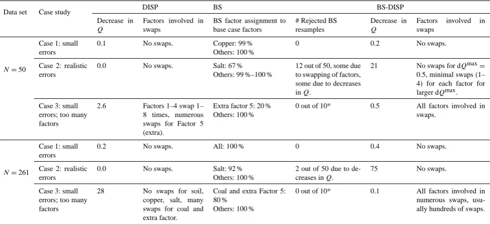
Table 1 summarizes the diagnostics reported by ME-2 for data sets with 50 or 261 samples. For brevity, detailed dis-cussion of these diagnostics is confined to the data sets with 50 samples. Diagnostic results were similar for the 261-sample data set. To put decreases ofQinto perspective, ro-bustQvalues for the data set with 50 samples were 500–600 for Cases 1 and 2 and 340 for Case 3. For the data set with 261 samples, robustQvalues were approximately 3000 for Cases 1 and 2 and 1800 for Case 3.
Decrease in Q for DISP. Small decreases inQ(less than 0.2) were reported for Cases 1 and 2, indicating that these solutions were global minima. A large value (greater than 2.5) was reported for Case 3, providing the first indication that there is something problematic with the modeling.
Table 1. Summary of error estimation diagnostics by data set and case study.
Data set Case study DISP BS BS-DISP
Decrease in Q
Factors involved in swaps
BS factor assignment to base case factors
# Rejected BS resamples
Decrease in Q
Factors involved in swaps
N=50
Case 1: small errors
0.1 No swaps. Copper: 99 % Others: 100 %
0 0.2 No swaps.
Case 2: realistic errors
0.0 No swaps. Salt: 67 % Others: 99 %–100 %
12 out of 50, some due to swapping of factors, some due to decreases inQ.
21 No swaps for dQmax=
0.5, minimal swaps (1– 4) for each factor for larger dQmax.
Case 3: small errors; too many factors
2.6 Factors 1–4 swap 1– 8 times, numerous swaps for Factor 5 (extra).
Extra factor 5: 20 % Others: 100 %
0 out of 10* 0.5 All factors involved in swaps.
N=261
Case 1: small errors
0.2 No swaps. All: 100 % 0 0.4 No swaps.
Case 2: realistic errors
0.0 No swaps. Salt: 92 % Others: 100 %
2 out of 50 due to de-creases inQ.
75 No swaps.
Case 3: small errors; too many factors
28 No swaps for soil, copper, salt, many swaps for coal and extra factor.
Coal and extra Factor 5: 80 %
Others: 100 %
0 out of 10* 0.1 All factors involved in numerous swaps, usu-ally hundreds of swaps.
* Used 10 bootstrap resamples because of the large number of factor swaps.
The extra factor (Factor 5) was involved in numerous swaps compared to the other factors, confirming that one too many factors was modeled. When only four factors, the true num-ber, were modeled for Case 3, the DISP diagnostics indicated no factor swaps.
Assigning BS Factors to Base Case Factors. All bootstrap factors were assigned to base case factors in 99–100 % of ev-ery bootstrap resample for Case 1. For Case 2, the salt factor was not consistently identified in 33 % of the resamples. This lack of reproducibility was likely caused by two compound-ing issues. One was that the factor was composed of just one species, Cl, with a small amount of EC. The other was that the factor’s contributions were defined by a few large values that could be excluded in BS resamples. For such resamples, this factor could be incorporated into other factors. For Case 3, all factors were reproduced in every bootstrap, except that Factor 5 (the extra factor that is comprised of small pieces of several species) was rarely found, confirming that one too many factors was modeled.
Decrease in Q and swapped factors in BS-DISP. In Case 1, no swaps occurred in the initial refitting of the full data set and no BS resamples were rejected because of swaps or large decreases inQ. This indicates that Case 1 was a well-defined PMF solution. For Case 2, diagnostics showed that 16 % of the resamples exhibited large decreases inQand 8 % con-tained swapped factors. The large decrease inQcompared to Case 1 is likely due to the larger data uncertainties used in Case 2. This indicates that Case 2 was not as well de-fined as Case 1, but there were few enough rejected ples that error estimates summarized for the accepted resam-ples were likely reliable and robust. For Case 3, all factors
were involved in numerous swaps, indicating serious prob-lems with the modeling and warning that interval estimates should not be interpreted.
4.2 Analysis of synthetic data sets – interval estimate examples
Output from DISP, BS, and BS-DISP includes interval esti-mates for each element for each factor and diagnostics for evaluating the trustworthiness of the interval estimates. As discussed in Sect. 3.2, estimates of intervals are calculated as follows: for DISP, endpoints of the uncertainty interval for a specific F factor element are the minimum value for that fac-tor element observed in all displacements and the maximum value for that factor element observed in all displacements. For BS, the endpoints of the uncertainty interval for a factor element are the 5th and 95th percentile values for that fac-tor element from all bootstrap resamples. For BS-DISP, each bootstrap resample is displaced and minimum and maximum values are calculated for each factor element as described for DISP. Then percentiles are taken across the resamples, the 5th percentile of the minima and the 95th percentile of the maxima, to create the final interval estimate.
Table 2a. Lower and upper interval estimates of PM2.5(µg m−3)by factor for Case 2 (realistic errors) for data sets with 50 or 261 samples.
Salt factor True PM2.5=0.10
Copper factor True PM2.5=0.42
Soil factor True PM2.5=1.82
Coal factor True PM2.5=2.24
Data set with 50 samples
DISP (0.00, 0.69) (0.12, 0.62) (1.23, 1.97) (2.08, 2.49)
BS (0.06, 0.75) (0.15, 0.69) (1.16, 1.90) (1.52, 2.38)
BS-DISP (0.00, 0.85) (0.12, 0.93) (1.17, 2.48) (1.54, 2.64)
Data set with 261 samples
DISP (0.06, 0.18) (0.33, 0.59) (1.59, 1.92) (2.08, 2.36)
BS (0.10, 0.28) (0.36, 0.54) (1.56, 1.82) (1.98, 2.27)
BS-DISP (0.07, 0.32) (0.33, 0.63) (1.52, 1.99) (2.00, 2.37)
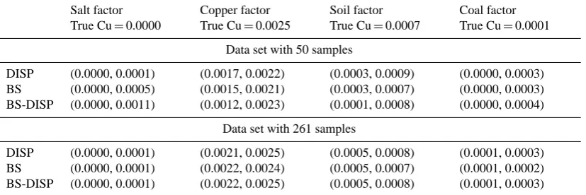
Table 2b. Lower and upper interval estimates of Cu (µg m−3)by factor for Case 2 (realistic errors) for data sets with 50 or 261 samples.
Salt factor True Cu=0.0000
Copper factor True Cu=0.0025
Soil factor True Cu=0.0007
Coal factor True Cu=0.0001
Data set with 50 samples
DISP (0.0000, 0.0001) (0.0017, 0.0022) (0.0003, 0.0009) (0.0000, 0.0003) BS (0.0000, 0.0005) (0.0015, 0.0021) (0.0003, 0.0007) (0.0000, 0.0003) BS-DISP (0.0000, 0.0011) (0.0012, 0.0023) (0.0001, 0.0008) (0.0000, 0.0004)
Data set with 261 samples
DISP (0.0000, 0.0001) (0.0021, 0.0025) (0.0005, 0.0008) (0.0001, 0.0003) BS (0.0000, 0.0001) (0.0022, 0.0024) (0.0005, 0.0007) (0.0001, 0.0002) BS-DISP (0.0000, 0.0001) (0.0022, 0.0025) (0.0005, 0.0008) (0.0001, 0.0003)
For PM2.5for the data set with 50 samples, the salt fac-tor’s overall contribution is uncertain, with possible values ranging up to 7 times the true amount. Comparatively, the soil and coal factors’ PM2.5mass estimates are more robust, with estimates ranging from about half of the true amount to just 10 % more for DISP and BS and 20–30 % more for BS-DISP. The copper factor is in between, with PM2.5 esti-mates ranging from a third of the true value to 1.5 to 2 times the true amount. The size of these intervals may seem large, but this data set contains just 50 samples. For comparison, intervals for the data set with 261 samples are included in the lower halves of Tables 2a and 2b. The markedly shorter intervals for the larger data set show the power of having more data. Intervals estimated from the smaller data set sup-port the idea presented in Sect. 1.6 about the sensitivity of BS to zero values in G, as evidenced by the long BS (and therefore BS-DISP) intervals compared to DISP. This differ-ence nearly disappears for the larger data set, supporting the idea presented in Sect. 1.4 that rotational uncertainty plays a lesser role in larger data sets.
For Cu, again the intervals for the larger data set are markedly shorter than those for the smaller data set. An-other note is that many of the intervals do not contain the true amount of Cu for the copper factor. That is, these error
methods do not always produce intervals that contain the true value.
4.3 Analysis of synthetic data sets – summary of comparisons
Table 3a. Summaries of F interval estimates for data sets with 50 observations.
Method for estimating intervals (number of bootstraps, dQmax)
First row: summary over all F factors
Second row: summary over all F factors excluding salt
(% coverage, median and avg ratios of length to middle of interval)
Case 1. Small errors Subset 1 Subset 2
DISP (n/a, 4) 98 %, 0.82, 1.04
98 %, 0.51, 0.86
100 %, 0.74, 1.00 100 %, 0.54, 0.85
BS (300, n/a) 77 %, 0.91, 1.05
73 %, 0.57, 0.88
73 %, 0.93, 1.00 71 %, 0.62, 0.87
BS–DISP (50, 0.5) 100 %, 1.28, 1.25
100 %, 1.01, 1.08
100 %, 1.25, 1.19 100 %, 0.93, 1.05
Case 2. Realistic errors
DISP (n/a, 4) 95 %, 1.49, 1.31
96 %, 1.03, 1.15
100 %, 1.47, 1.32 100 %, 0.93, 1.16
BS (300, n/a) 78 %, 1.53, 1.36
81 %, 1.16, 1.23
81 %, 1.39, 1.24 79 %, 0.82, 1.06
BS–DISP (50, 0.5) 97 %, 2.00, 1.54
96 %, 1.59, 1.39
98 %, 1.74, 1.36 98 %, 0.98, 1.21
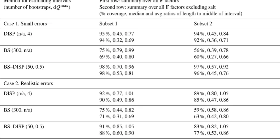
Table 3b. Summaries of F interval estimates for data sets with 261 observations.
Method for estimating intervals (number of bootstraps, dQmax)
First row: summary over all F factors
Second row: summary over all F factors excluding salt
(% coverage, median and avg ratios of length to middle of interval)
Case 1. Small errors Subset 1 Subset 2
DISP (n/a, 4) 95 %, 0.45, 0.77
94 %, 0.32, 0.69
94 %, 0.45, 0.84 92 %, 0.36, 0.71
BS (300, n/a) 75 %, 0.79, 0.99
69 %, 0.40, 0.80
56 %, 0.39, 0.78 60 %, 0.27, 0.66
BS–DISP (50, 0.5) 98 %, 0.70, 0.96
98 %, 0.53, 0.81
97 %, 0.57, 0.92 96 %, 0.45, 0.76
Case 2. Realistic errors
DISP (n/a, 4) 92 %, 0.77, 1.01
90 %, 0.49, 0.86
89 %, 0.80, 1.05 85 %, 0.47, 0.86
BS (300, n/a) 75 %, 0.44, 0.82
71 %, 0.31, 0.69
59 %, 0.58, 0.86 63 %, 0.42, 0.80
BS–DISP (50, 0.5) 91 %, 0.85, 1.05
88 %, 0.60, 0.90
83 %, 0.82, 1.05 77 %, 0.53, 0.86
To test repeatability of results, two replicates of each data set were generated and modeled. The original data set con-tained 783 observations. For the 261-day replicates, every third sample was retained, starting with the first sample for Subset 1 and the second sample for Subset 2. For the 50-day replicates, every 15th sample was retained, starting with the first sample for Subset 1 and the second sample for Subset 2. DISP results are presented only if no swaps occurred and if
in table cells) and also over all factors excluding the sea salt factor (lower row) since modeling of bootstrapped resamples did not always fit a factor highly correlated with the sea salt factor (as described in Table 1). Case 3, the case in which modeling error was introduced, was excluded from this sum-mary analysis since diagnostics for this case indicated prob-lems, as discussed in Sect. 4.1. Results are presented in Ta-bles 3a and 3b.
These summaries show that percent coverage is generally high, greater than 90 %, except for BS and for BS-DISP with the larger data set for Case 2. Also, DISP generally provides the shortest intervals, except for Case 2 with the larger data set, where BS provides the shortest intervals.
Results from Subset 1 and Subset 2 are similar for DISP and BS-DISP. Unexpectedly, BS results vary by subset. The reason is unclear at this time, but it may have to do with the number of zeros in G for the two subsets. For the data set with 50 samples, Subset 1 has 3, 3, 7, and 1 zeros and Subset 2 has 1, 6, 12, and 1 zeros for coal, salt, copper, and soil fac-tors, respectively. For the data set with 261 samples, Subset 1 has 6, 17, 27, and 8 zeros and Subset 2 has 5, 26, 44, and 7 ze-ros for coal, salt, copper, and soil factors, respectively. It does not take many zeros to reduce rotational uncertainty; thus, the larger number of zeros for Subset 2 of the smaller data set could explain the shorter intervals. The cause for lower percentage coverages for BS for Subset 2 is unknown.
As expected and seen with the examples presented in the previous section, it is noted that intervals are shorter for the larger data set. This is true for all methods and both case studies. What is not expected is that percentage coverage is lower for the larger data set. The cause is unclear; however, a proposed explanation is that the likelihood of excessively long intervals is higher for smaller data sets because there are fewer zeros in G. These excessively long intervals will in turn result in unnaturally high coverage.
The conclusion from the analysis of these synthetic data sets is that DISP consistently provides intervals that have high coverage (>90 %) and that are shorter than those pro-vided by BS or BS-DISP. BS-DISP sometimes provides in-tervals with higher coverage than DISP, but these inin-tervals are generally longer. The performance of error estimation techniques will depend on the details of each individual data set. Here, the differences seen for supposedly similar case studies 1 and 2 illustrate the variability found between data sets.
Although patterns in relative merits of the three uncer-tainty estimation techniques are developing, applying these inferences to all PMF analyses is premature. Variation in characteristics of data sets (e.g., number of samples, num-ber of zeroes in G) and modeling errors (e.g., inappropriate number of factors, discrepancies betweensij anduij, han-dling of values below method detection limit) may lead to different relative merits. In order to achieve the best possi-ble uncertainty estimations, the evaluation approach of this paper should preferably be repeated whenever PMF error
estimation is applied to new kinds of data sets: simulations with realistic true data patterns should be performed and mer-its of uncertainty estimates should be evaluated. A forthcom-ing manuscript (Brown et al., 2014) will present case studies of ambient data and interpretation of results from the three error estimation techniques.
5 Reporting recommendations for PMF analyses
Reff et al. (2007) performed a literature review of publica-tions of PMF applicapublica-tions. The purpose of the review was to document the numerous decisions that users of PMF must make to perform such applications and to encourage that fu-ture publications of PMF applications include enough details for readers to evaluate, reproduce, or compare results be-tween different studies. In a continuing effort to help make the reporting of results from EPA PMF and ME-2 more sys-tematic among researchers, we have summarized recommen-dations on what to report while documenting uncertainty es-timates from PMF analyses. This is not an exhaustive list, and every data set may require that additional information be reported. To increase the understanding of the behavior of these uncertainty estimates with different types of data, it is recommended that all three techniques be applied and spe-cific details about and estimated intervals from each method be reported. For cases where this is not possible or reason-able, it is recommended that such reasoning be included in the publication.
BS. Report the number of resamples analyzed and the size of percentiles of the obtained distribution of results chosen for error limits, e.g., 5th and 95th percentiles. Also report the percentage of BS factors assigned to each base case factor and the number of BS factors not assigned to any base case factor.
DISP. Report species not displaced such as those down-weighted, the absolute and relative decrease inQ, and the number of factor swaps. If factor swaps occur for the small-est dQmax, it indicates that there is significant rotational am-biguity and that the solution is not sufficiently robust to be used. If the decrease inQis greater than 1 %, it likely is the case that no DISP results should be published unless DISP analysis is redone after finding the true global minimum of
Q.
BS-DISP. As with BS and DISP, report the number of BS resamples analyzed, the size of percentiles chosen for error limits, the species actively displaced, the decrease inQ, and the number of factor swaps.
6 Conclusions
addition to those reported in this work. All indicate that if data uncertainties are known and there are no modeling er-rors, then the DISP method consistently produces good cov-erage of true values using the shortest possible uncertainty intervals. In the more difficult cases where data uncertain-ties are not well known, the bootstrap-based methods BS and BS-DISP seem to work satisfactorily, provided that there are no modeling errors. A solution’s stability can also be eval-uated via the fraction of times each factor is mapped in BS and if any swaps occur in DISP. These results provide critical information on whether a solution should be interpreted.
The uncertainty estimation with DISP depends on the user’s defined maximum allowed change inQ(dQmax). For simulated data, this dependence was illustrated in this work. For real data, mathematical derivation is impossible because of the presence of modeling errors. Practical experience is needed in order to understand the dependence on dQmax. Such understanding might be attempted by partitioning a real data set in various ways and comparing the partition-partition variation of profiles against their DISP uncertainty estimates. In a companion paper, to be submitted soon, several real-data analyses will be reported. It should be noted that the dependence of uncertainty intervals on dQmax depends on the amount of rotational ambiguity. If the model has no ro-tational ambiguity, then uncertainties computed by DISP are expected to be proportional to square root of dQmax. At the other extreme, if the rotational uncertainty is dominant, then the computed uncertainties are expected to be almost inde-pendent of dQmax. In EPA PMF, the DISP method is imple-mented so that uncertainties are always computed for four different dQmaxvalues. In this way, the influence of dQmax
values on uncertainty estimates is easy to see for each spe-cific data set.
In order to speed up computations, some factor elements may be defined as passive in DISP and BS-DISP processes. Defining some elements as passive has no influence on the uncertainty intervals obtained for active (actively displaced) factor elements. Uncertainty intervals for active factor ments are reliable regardless of how many and which ele-ments are defined as passive, provided the user-provided data uncertainties and dQmaxare correct. Thus it is safe to define uninteresting factor elements as passive in order to speed up computations. Note though that defining a factor element as passive will usually underestimate its computed uncertainty. Specifically, the uncertainty for a factor element defined as passive will be less than or equal to the uncertainty computed for that factor element if it were defined as active. Thus factor elements critical for associating a factor with a source should always be defined as active.
The present work offers no quantitative results for the sit-uations where significant modeling errors exist. It was seen that one type of modeling error, specifying more factors than the data support, leads to diagnostics that suggest to an at-tentive PMF user that there are too many factors. However, it is not currently known whether diagnostics will be as clear
if multiple modeling errors are present. For example, censor-ing a large number of values below detection limit, another type of modeling error, may invalidate uncertainty analysis by BS, DISP, and BS-DISP.
It was seen that some data sets produce large rotational uncertainties for some or all factors so that interval estimates may extend down to zero even for some of the defining “key” species. In such cases, factor identities may become fluid, often indicated by factor swaps. The obtained uncertainty in-tervals are then imprecise because of the difficulty of defin-ing the borderline between rotations and swaps. Although the methods will correctly indicate that uncertainties are large, they may not produce quantitative results for these large in-tervals. On the other hand, this “weakness” caused by factor swapping may not be important in practical work. Simply put, it does not matter whether uncertainty is rather large or very large.
When interpreting large uncertainties, there is a concep-tual issue that warrants highlighting. Suppose a factor is as-sociated with a known source or sources based on the initial computed composition. For example, suppose factor F1 is identified as “Diesel vehicles” based on a high value of EC. Now suppose that the estimated uncertainty for EC for fac-tor F1 shows that there may be low or no EC apportioned to the factor. This would then call into question the asso-ciation of this factor with the postulated source. Therefore, when discussing uncertainties, they should be called uncer-tainties in factor F1, not unceruncer-tainties in the diesel factor. If the uncertainties are small enough that the source or sources associated with a factor are not called into question, then it is reasonable to refer to the uncertainties as uncertainties in the source profile. When reporting results, it is important to document each factor for which the size of the uncertainties calls into question the source or sources initially associated with that factor.
If large uncertainties are obtained for a PMF solution, the next step is for the analyst to determine whether physical-chemical arguments can be applied to reduce the variability of the results. Different constraints can be defined, for exam-ple, by constraining certain G or F factor elements to be zero (Paatero et al., 2002). Narrower uncertainty intervals will be obtained. However, no results from such experiments are in-cluded in this work.
It has been customary to report uncertainties in the sym-metric form, as “best fit±uncertainty”. In the present case, such a formulation is not adequate since uncertainty intervals need not be symmetric. Uncertainties should be reported in an unsymmetrical formulation, for example, as “best fit +