Integrated planning of electric vehicles routing and charging stations location considering transportation networks and power distribution systems Pages 535-550 Download PDF

(1)

* Corresponding author

E-mail: [email protected] (M. Granada)

2018 Growing Science Ltd. doi: 10.5267/j.ijiec.2017.10.002

International Journal of Industrial Engineering Computations 9 (2018) 535–550

Contents lists available at GrowingScience

International Journal of Industrial Engineering Computations

homepage: www.GrowingScience.com/ijiec

Integrated planning of electric vehicles routing and charging stations location

considering transportation networks and power distribution systems

Andrés Ariasa, Juan D. Sancheza and Mauricio Granadaa*

a_{Program of Electrical Engineering, Technological University of Pereira, Pereira, Colombia}

C H R O N I C L E A B S T R A C T

Article history: Received June 18 2017 Received in Revised Format August 25 2017

Accepted November 7 2017 Available online

November 7 2017

Electric Vehicles (EVs) represent a significant option that contributes to improve the mobility and reduce the pollution, leaving a future expectation in the merchandise transportation sector, which has been demonstrated with pilot projects of companies operating EVs for products delivering. In this work a new approach of EVs for merchandise transportation considering the location of Electric Vehicle Charging Stations (EVCSs) and the impact on the Power Distribution System (PDS) is addressed. This integrated planning is formulated through a mixed integer non-linear mathematical model. Test systems of different sizes are designed to evaluate the model performance, considering the transportation network and PDS. The results show a trade-off between EVs routing, PDS energy losses and EVCSs location.

Keywords:

Electric Vehicle

Capacitated Vehicle Routing Problem

Transportation network, power distribution system

Electric Vehicle Charging Station

1. Introduction

In the last years, the reduction of the negative impact on the environment produced by the transportation sector has been identified as a relevant issue. According to surveys of Environmental Protection Agency, release of Green House Gases (GHG) provided by the non-renewable energy sources and its derivatives, contribute to 14% of the global pollution (Intergovernmental Panel on Climate Change. Working Group III and Edenhofer n.d.). As established in the road map of Energy Technologies Perspectives, carbon dioxide emissions will be reduced up to 50% by 2050, compared to levels presented in 2005. The 30% of this reduction depends directly by the transportation sector, due to a high penetration of Electric Vehicles (EVs) forecasted by 2050 worldwide and the friendly alternative that this transportation mean can provide to the environment, in comparison with vehicles propelled by internal combustion engines (Tanaka, 2011). Due to the low efficiency of internal combustion engines and increase of cities urbanization rate, EV has become into a more attractive transportation mean, granting possible solutions to worldwide problems that involve the environment, electric power supply and mobility. Some of the advantages provided by EVs are listed below:

(2)

 Permit to obtain a balance close to zero in carbon dioxide emissions release, from the electric power generation source to the EV tire, as long as the electricity has been generated with renewable sources.

 Provide a significant noise reduction.

 Contribute to the expansion of Smart Grid concept, considering decentralized energy storage and

demand response.

 Accelerate the development of policies that stimulates the hourly tariff implementation, as a result

of the reinjection of the energy stored in the EVs to the Power Distribution System (PDS), applying V2G (Vehicle to Grid) concept.

Since the point of view of the cost-benefit relationship, EVs are not as competitive as conventional vehicles are; respect to drive range, costs and availability of refueling stations. This overview may change at short term due to penalization policies imposed for overcoming the limit of GHG. In this regards, from 2019, European Union will impose a 95 Euros fine to vehicles with emissions greater than 147 grams of CO2 per kilometer traveled (Mock, 2014). During the last decades, the EVs population has been increased rapidly, and its development has reached great maturity (Chan, 1999). Some studies estimate that by 2030 the proportion of EVs will be around 64% of the total of light vehicles (Du et al., 2010). In the transportation sector, the companies are highly responsible to reduce the GHG emissions, emerging several pilot projects for load transportation with EVs in multinational companies such as DHL, FedEx and UPS, where EVs have been included for routing planning.

Despite the above, the emerging of EVs as the main transportation mean is still overshadowed by the low driving range (in comparison with internal combustion engines vehicles), provided by the lithium-ion batteries that lead the EVs energy storage market. The improvement for this type of batteries, in terms of driving range increase, is greatly hampered by issues related with safety, cost, operation temperature and availability of materials (Hannan et al., 2017), which implies that the EVs driving range will not widely improve for the coming years.

Under these circumstances, charging stations play an important role on the electric mobility, allowing to travel longer distances by indirectly increasing EV driving range. In this manner, it is necessary to perform an appropriate siting of Electric Vehicle Charging Stations (EVCSs), as this type of installations are strategic for the massive incorporation of EVs, reaching driving ranges comparable with conventional vehicles. Furthermore, optimal siting of EVCSs does not depend exclusively on the transportation network requirements, because those installations imply large consumptions of electricity. Therefore, the effect of the charging stations on the power distribution networks has to be taken into account, in order to avoid congestion or additional costs associated with energy losses.

(3)

A. Arias et al.

Other important publications can be found, such as (Shojaabadi et al., 2016) where the optimal planning of EVCSs is done considering customer’s participation in demand response programs and uncertainties associated with load values, arrival time of EVs to EVCSs, initial state of charge of EVs’ batteries and electricity market price. Based on a shared nearest neighbor clustering algorithm and queuing theory, the authors in (Dong et al., 2016) have developed a planning method, which is decomposed into three parts: a spatial-temporal model of EVs charging points, a location determination model and a capacity determination model. Distribution network is not taken into account in the planning method, due to the long distance between any two EVCSs and each of them is supplied by a separate distribution network. In contrast with (Dong et al., 2016), in (Luo et al., 2015) the PDS and transportation network graphs are considered, in conjunction with EV owners, urban infrastructure and EVCSs. This way, a multi-stage charging station placement strategy with incremental EV penetration rates is formulated, applying a Bayesian game framework to analyze the strategic interactions among EVCSs service providers.

In this work, the Electric Vehicles Integrated Planning Problem (EVs-IPP) for cargo transportation is presented. The optimal location of EVCSs is performed considering the mobility of cargo EVs along the transportation network and the impact on the PDS. This results as a consequence of the poor capacity that may be presented on the EVs’ battery to provide enough autonomy to complete the routes adequately, since the EVs are part of merchandise transport where considerable distances are traveled too often. By the other side, EVCSs represent huge additional loads for the electric network, being the proper location of this type of loads a critical aspect when the energy losses of the PDS are assessed.

A mixed integer non-linear mathematical model is proposed to portray the EVs mobility with the well-known Capacited Vehicle Routing Problem (CVRP) and the distribution system operation with the power flow equations. In this manner, costs associated with cargo EVs routing, EVCSs installation and energy losses are minimized, obtaining an optimal operation in the transportation and electric networks. Additionally, the introduction of a consistent penalty in the objective function helps to determine until what level the current EVs’ battery autonomy is suitable to perform the routes. Regardless the battery autonomy, the mathematical model tends to be feasible, as long as this term is not greatly weighted in the objective function. This way, under a non-sufficient battery autonomy scenario, the decision maker can realize that EVCSs installation is not enough to meet the needs of EVs routing, being necessary to replace current batteries for others with larger drive range.

This paper is organized as follows: Section 2 shows the proposed mathematical model of EVs-IPP. Later, section 3 details the test systems used to evaluate the EVs-IPP performance, coupling instances of transportation networks and PDS from the specialized literature. In section 4, the results for different scenarios are depicted. Finally the conclusions of the work are presented in section 5.

2. EVs-IPP formulation

The integrated planning problem proposed in this work, can be formulated as a graph theory problem.

Let G=(V,A) a complete graph, where V=C∪N is the vertices set of the integrated problem and A is the

arc set that interconnects all the vertices. Set C={1,…,c} represents the customers vertices and conform

the cargo transportation network. Set N={c+1,…,c+n} represents the power demand vertices and

conform the PDS. Set J⊆N contains all the candidate vertices to install EVCS that in this case is the set

of all the nodes except the PDS substations. Sets N and C and their respective arcs can be seen as two

disjunctive graphs, and the interaction between these graphs is given by the EVs charging. The EVs are

required to meet the customers merchandise demand. PDS vertices of set N are connected each other

through lines, which represent the electrical wires, conforming set L={1,…,l}.

(4)

vehicles have to fully meet the merchandise demands, seeking a travelling minimal cost (Christofides, Mingozzi, and Toth 1977). The second subproblem is related with the location of EVCSs, which indirectly provides an increase of the EVs battery range in order to complete the travel satisfactorily. The third subproblem frames the power flow formulation, involving the operation point of the PDS under the additional loads represented by the EVCSs installed.

2.1 Nomenclature

For clarification, the notations used in this paper are listed as follows.

Sets:

C Set of customers

J Set of candidate nodes to install _EVCSs

{0} Depot

{0’} Copy of Depot

V {C}∪{J}∪{0}∪{0’}

K Set of electric vehicles

N Set of nodes belonging the PDS

L Set of lines belonging the PDS

Parameters:

1

W Weight factor for EVCSs installation cost term

2

W Weight factor for routing cost

3

W Weight factor for penalization term

4

W Weight factor for energy losses cost

h

f EVCS installation cost [USD]

h

fm EVCS maintenance cost [USD]

CPI Consumer Price Index

nt Number of years to shift to future value

k

a Cost per kilometer traveled of vehicle k [USD/km]

gh

d Distance between node g to node h [km]

k

am Maintenance cost of vehicle k to travel one kilometer [USD/km]

k

ap Cost of the additional capacity of the EV’s battery [USD/km]

b Cost of 1 kWh of energy losses [USD/kWh]

/

w oEVCSs

Loss Power losses of the PDS without EVCSs installed [kW]

M Big number

|K | Cardinality of set K

g

q Merchandise demand at customer node g

k

U Merchandise cargo capacity of vehicle k

Q Battery autonomy [km]

d n

P Active power demanded at node n [kW]

mn

R Resistance of line mn belonging the PDS [Ω]

mn

X Reactance of line mn belonging the PDS [Ω]

mn

Z Impedance of line mn belonging the PDS [Ω]

min

(5)

A. Arias et al.

max

V Upper level of voltage at PDS nodes [V]

max

I Upper level of current at PDS lines [A]

maxG

P Upper level of active power generated at PDS nodes [W]

PEVCS Nominal Active power drawn by EVCS installed [kW]

Variables:

 Cost of EVCSs installed [USD]

 Cost of EVs routing at transportation network [USD]



Cost of penalization [USD]

 Cost of energy losses at PDS [USD]

h

y Binary decision variable for EVCS installation at candidate node h. If

yh=1 the EVCS is installed and yh=0 otherwise

ghk

x Binary decision variable, taking a value of 1 if vehicle k goes from node

g to node h and 0 otherwise

ficticious hk

P Missing autonomy to reach node h with vehicle k [km]

sqrt mn

i Square current flowing through line mn of PDS [A2_]

ghk

u Remaining merchandise when vehicle k leaves node g and goes to node

h

1 hk

pb Battery autonomy before vehicle k arrives node h [km]

2

gk

pb Battery autonomy after vehicle k leaves node g [km]

mn

P Active power flowing line mn of PDS [kW]

G n

P Active power generated at node n [kW]

n

PE Active power drawn by an EVCS installed at node n [kW]

mn

Q Reactive power flowing line mn of PDS [kVar]

G n

Q Reactive power generated at node n [kVar]

sqr m

V Square voltage at node m [V2_]

2.2 EVs-IPP Mathematical Model

The mathematical model for EVs-IPP is presented in equations (1) to (29), considering {0} as the depot where the vehicles start the respective routes and {0’} is a depot copy where the vehicles will complete the routes.

1 2 3 4

min z W        W  W  W  ₍₁₎

Subject to:



_h _h



_h



1



nt

h J

f fm y CPI

 





    ₍₂₎



 



365 _k _gh _ghk 1 _k 1 nt

g V h V k K

a d x am CPI



  

 



      ₍₃₎





365 ficticious 1 nt

k hk

h V k K

ap P CPI



 

 



   ₍₄₎



w/o EVCSs







8760 sqrt 1 nt

mn mn

mn L

b i R Loss CPI





 



   

(5)

\{ '},

1

ghk g V o g h k K

x

  



 

 h C

(6)

\{ '} ghk h g V o g h k K

x M y

  

 

 

 h J

(7)

\{ }, \{ '},

0

ghk ghk

h V o h g h V o h g

x x

   

 



 g V\ { , '},o o  k K

(8)

'

\{ } \{ '}

0

ohk ho k h V o h V o

x x

 

 



 k K

(9)

\{ }

1

ohk h V o

x







 k K

(10)

\{ }

| |

ohk k K h V o

x K   

 

(11)

\{ ', } ghk \{ , } hgk g V o j g V o j

u u   



,

h J k K

   

(12)





\{ , } \{ ', } \{ ', }

1

ghk hgk g hgk k hgk

h V o g h V o g h V o g

u u q x U x

         _  _  



, g C k K    

(13)

0



u

ghk



U x

k



ghk g V o h V\ { '},  \ { },o g h k K ,  (14)

1 2 ₍₁ ₎

hk gk gh g hk g hk

pb pb d x Q x  g V \ { '},o h V \ { '},o gh k, K ₍₁₅₎

2

ok k K

pb



Q

  (16)

2

gk g

pb  Q y  g J ₍₁₇₎

2 1 ficticious hk hk hk

pb  pb  P  h C (18)

1

₀

hk

pb



 h V (19)

, {0,1}

j ghk

y x     j J g V, \ { '},o  h V\ { },o  k K ₍₂₀₎

( sqrt ) G d

mn nr nr nr n n n

mn L nr L

P P i R P P PE

 

     



 m N, n N, r N ₍₂₁₎

( sqrt ) G d

mn nr nr nr n n

mn L nr L

Q Q i X Q Q

 

    



 m N, n N, r N ₍₂₂₎

2

2( )

sqr sqr sqr

m n mn mn mn mn mn mn

v v  R P X Q Z i mnL, m N, n N (23)

2 2

sqr sqr

n mn mn mn

v



i



P



Q

mnL, n N (24)

2 2

min max

sqr n

V



v



V

 n N (25)

2 max

0

sqr mn

i

I



mnL (26)

max

0

G G

n

P



 n N (27)

.

n h

PE PEVCS y  n N  h J  n N, j N (28)

0

h ficticia

P   h V ₍₂₉₎

The objective function in Eq. (1) seeks to minimize the summation of four terms. The first term is the

construction and maintenance cost of an EVCS at node h. The second term is the routing cost performed

by the vehicle k from node g to node h. In this term the maintenance in terms of the distance traveled by

the EV is also considered. The third term is a penalization created in case of need to increase the battery autonomy in EVs, in order to complete the routing and deliver the merchandise to customers. This term

is the cost to make the problem feasible and is defined as the product between a positive variable ficticious

hk

P

(Increase of the battery autonomy at vehicle k to arrive node h) and the cost apk of the additional capacity

(7)

A. Arias et al.

terms of the objective function are defined in Eqs. (2-5) respectively, along a period equal to one year

and shifted to future value. This latter depends on the number of years nt the cost will be shifted to future

and the Consumer Price Index CPI. Weighting factors W1, W2, W3 and W4 in objective function provide

a level of importance for each term, making the summation of all of them equals to the unity. The values assigned to these factors depend on strategic data managed by decision maker in the integrated planning. This information is related with financial availability to implement the routing, EVCSs construction, battery technology, between others. The values that best represent the deal between objectives can be obtained via a multi-objective approach, in order to build up an optimal front of solutions (which is not into the scope of this work). In the proposed model, punctual values for these factors are used in all instances and runs, distributing the relative importance of each factor in objective function, in such a way that the need to increase the battery autonomy is largely penalized and the routing cost is of greater

importance than EVCSs installation and energy losses costs. Thus, in this proposal it is assumed that W3

>W2 >W1 =W4. Factor W3 has the highest relevance, as it is attempted that a change of the battery capacity

is not attractive. W2 is greater than W1 as the solution space of the routing is less restricted than the

solution space of the EVCSs installation. Therefore, the aim is to prioritize routing over the EVCSs installation.

The constraint in (6) requires every arc to be traveled only once, while constraint in Eq. (7) is an inequality to warranty that EVs only recharge their batteries at a located EVCS. Eq. (8) is a constraint that assures the flow for each vehicle at each node. In (9), it is shown that the quantity of vehicles leaving the depot has to be the same as the number of vehicles entering the depot. Constraint in Eq. (10) requires

each vehicle to do one trip at most. In (11), the cardinality of set K, assures that the maximum quantity

of vehicles leaving the depot is limited by the quantity of vehicles available.

When vehicles visit an EVCS without merchandise demand, qh=0, hϵJ. Constraint in Eq. (12) represents

that the summation of the remaining load ughk of an EV entering an EVCS is equal to the remaining load

of the vehicle leaving an EVCS. This guarantees the vehicle capacity balance and indicates that an EVCS can be revisited more than once. The change in the remaining load of an EV when entering a customer

node (with qh≥0) is calculated by constraint (13). If the vehicle k visits customer h, the remaining cargo

is reduced by customer demand qh. If the customer h is not visited by vehicle k, the constraint keeps valid.

Both, constraints in (12) and (13) make an EV to pass by an EVCS more than once but visit a customer

only once, and eliminate the generation of subtours. Constraint in (14) contains the range for ughk that

can be at most, the total cargo capacity of the EV. Since the point of view of the EV battery, constraint

in (15) records the EV battery autonomy in terms of distance. When the vehicle k with a battery autonomy

Q, travels along the arc gh, the battery autonomy before entering node h 1

hk

pb , is the subtraction between

the battery range after leaving node g 2

gk

pb and the distance traveled dgh along the arc.

Constraint (16) indicates that all the vehicles have to leave the depot with batteries completely charged. This also applies for the EVCSs, where constraint (17) describes that a vehicle will have its battery fully charged once leaving from the EVCS. Right before an EV enters a customer node, the battery autonomy will be the same once it leaves the node, which is established in constraint (18). If the vehicle does not

have enough autonomy to arrive to the next node, a variable called ficticious

hk

P is in charge to provide the

missing autonomy. This latter is introduced in the objective function as a penalization, motivating the installation of EVCSs instead of to increase the EVs battery autonomy. In Eq. (19) the non-negativity of the battery autonomy is declared, and the binary decision variables are shown in Eq. (20). From Eq. (21) to Eq. (27) the status of the PDS is assessed. The balance of active and reactive power is done in Eq. (21)

and Eq. (22) respectively. The voltage drop along the network segment mn is computed in (23) and the

current square is obtained with constraint (24). The constraints from (25) to (28) determine the voltage limits for each node, current flowing through the lines, active power generated and power consumed by

the EVCSs, being PEVCS the maximum power consumed by each EVCS. The non-negativity of the

(8)

3. Test systems and EVS-IPP mathematical model validation

In order to validate the mathematical model proposed, three different instances composed by combination of transportation networks and power distribution systems from the specialized literature are proposed. The characteristics of the transportation, power distribution and hybrid networks, are featured below. Some tests are carried out on the uncoupled instances.

3.1. Transportation networks test systems

In this study, small-size instances for CVRP are used to examine the EVs-IPP mathematical model since the transportation network approach. As shown in (Yang and Sun 2015), three instances are generated

from the Pn16k8 instance, available in (NEO Networking and Emerging Optimization 2013). Instead of

using all customers in the instance, each instance contains only a certain number of customers. For

example, in this work, Pn6k2 presents the last 6 customers of Pn16k8, Pn7k3 presents the last 7 customers

of Pn16k8 with 3 vehicles, and Pn8k3 contains the last 8 customers of Pn16k8 with 3 vehicles (Table 1).

According to the tests performed in (Yang and Sun 2015), the autonomy Q for the EV’s battery is set in

[1.2dmax], being dmax the maximum Euclidean distance between any two nodes in the network. The cost

associated with an EVCS construction is [0.5Q]. In this case, it is assumed that all the customer nodes

are candidates for EVCSs.

Table 1

Small-size transportation network instances

Instance _{Coord.X Coord.Y}

Pn6k2 Pn7k3 Pn8k3

Customer node

EVCS candidate

node

Customer

node candidate nodeEVCS Customer node1 EVCS candidate node 9 57 58

1 8 2 10 62 42

1 7 2 9 3 11 42 57

2 8 3 10 4 12 27 68

3 9 4 11 5 13 43 67

4 10 5 12 6 14 58 48

5 11 6 13 7 15 58 27

6 12 7 14 8 16 37 69

Depot (0 and 0’) 1 -1

Table 2 provides the results obtained by EVs-IPP in Pn6k2, Pn7k3 and Pn8k3 instances, which can also

be found in (Yang and Sun 2015). Note that the candidate nodes where EVCSs were installed at are underlined along the EVs routes described in the column “Route”.

Table 2

Results for three different transportation network instances

Instance EVCSs installed

Objective function

Route _{Time [s]}

k=1 k=2 k=3

Pn6k2 2 426.8609 0-10-4-5-0’ 0-1-9-3-6-2-0’ 21

Pn7k3 2 428.5961 0-6-1-12-5-0’ 0-3-7-14-4-2-0’ 688

Pn8k3 2 597.1575 0-4-16-8-5-3-0’ 0-7-2-14-0’ 0-1-6-14-0’ 352

3.2. Power distribution test systems

(9)

A. Arias et al.

Considering the effect of the power distribution system in EVs-IPP mathematical model, the electric feeders mentioned above are coupled with a transportation network. No matter which transportation

network is used for this test, if a big autonomy Q for the EVs’ batteries is used, the vehicles are able to

complete the routes and meet the customers, without the need to install any EVCSs. In this sense, the results (voltage profile) since the point of view of the power distribution system will be quite similar as those that can be obtained with the conventional back-forward sweep algorithm, as there are no additional power loads. The error in p.u. between the voltage calculated by back-forward sweep algorithm and the EVs-IPP mathematical model is shown in Figs. 1-3 for DS16N, DS34N, DS23N test systems respectively.

Fig. 1. Voltages error in p.u. for DS16N test system between backward-forward sweep algorithm and EVs-IPP mathematical model

Since the lower limit of voltage constraint in EVs-IPP mathematical model is not reached, the voltage at nodes are very similar compared with the voltage obtained with backward-forward sweep algorithm, as this latter is not able to restrict this variable. Figs. (1-3) depict that the maximum error between the two

methods is 1.9928 x 10-9_.

3.3. Coupled systems

In order to examine the EVs-IPP’s capability from a general perspective, both electric and transportation networks are coupled. Therefore, three new instances are created from the power networks and transportation instances shown before. These new instances are exposed in detail in (Power Systems

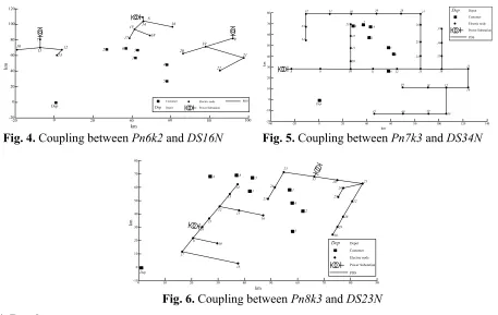
Planning Group n.d.). Fig. 4 shows the coupling between Pn6k2 and DS16N. Note that nodes joined with

continuous line represent the power distribution system, being nodes 7, 8 and 9 the distribution substations. The transportation network is portrayed by the square nodes. Fig. 5 presents the coupling

1 2 3 4 5 6 7 8 9 10 11 12 13 14 15 16 Node

E

rror p.

u.

10-14

10-15 10-13 10-12 10-11

1 2 3 4 5 6 7 8 9 101112 13 14 15 1617 18 1920 21 2223 242526 2728 29 3031 3233 34 0.4

0.6 0.8 1 1.2 1.4 1.6 1.8 2x 10

-9

Node

E

rror p.

u.

1 2 3 4 5 6 7 8 9 10 11 12 13 14 15 16 17 18 19 20 21 22 23 Node

0.5 1 1.5 2 2.5 3x 10

-13

E

rror p.

(10)

between Pn7k3 and DS34N, where node 8 is the distribution substation. Finally, coupling of Pn8k3 and

DS23N is shown in Fig. 6, with two distribution feeders around the transportation network compound by

8 nodes. In all three instances, it is assumed that none of the PDS nodes is located at the same coordinates of the customers. Therefore, EVCSs are not able to be installed on the customers’ nodes (as EVCSs draw power from electric grid), which implies that the EV is required to visit a power network node (to an installed EVCS) once the battery is almost depleted and returns to still visiting the customers.

Fig. 4. Coupling between Pn6k2 and DS16N Fig. 5. Coupling between Pn7k3 and DS34N

Fig. 6. Coupling between Pn8k3 and DS23N

4. Results

Coupled systems shown in Figs. (4-6), are utilized to assess the performance of EVs-IPP. Parameters for all three instances were chosen consistently to the reality. According to (Tesla Supercharger 2017), an

EVCS may draw from the PDS up to 120 kW for a 272 km battery-range. In this work, PEVCS used is

60 kW, as the average range evaluated in the runs is around 130 km, considering a linear behavior

between maximum power at EVCS and distance that can be traveled. The cost fh related with EVCS

construction is assumed to be 22000 USD, as established in (Agenbroad 2014), taking into account type

of installation, materials, connectivity, data and other factors. Parameter fmh, which is the maintenance

cost associated with this infrastructure, is around 10% the installation cost. Since the point of view of the EV operation, the average cost is 2.423 USD to travel 100 km, as reported by (U.S. Department of Energy

2017), and an estimation of 86 USD for EV maintenance every 5000 km traveled. The parameter apkis

chosen arbitrarily as 1000 times the cost per kilometer travelled, in order to strongly penalize the third term in the objective function. By the hand of PDS losses, the power losses cost used in all cases is 4.34

Cents per kWh. To shift the cost to future value, CPI is set in 5%. Weighting factors assigned in the

objective function at all runs are: W1=0.1, W2=0.2, W3=0.6 and W4=0.1. There is a high weight for the

third term in objective function, in comparison to the other terms, as the purpose is to obtain a solution where the EVCSs installation be encouraged instead of change the EVs’ battery for a battery with larger

autonomy. The proposed EVs-IPP model has been programmed and executed in the GAMS (General

Algebraic Modeling System) environment (GAMS Development Corporation 2016) on a HP desktop

computer, Windows 64-bit operating system, with an Intel Core i3 @ 3.3 GHz processor and 4 GB of RAM. The presence of nonlinearities and integer and continuous variables into equations, make the proposed EVs-IPP model be a MINLP, which is solved using the DICOPT solver (GAMS Development Corporation 2016). Dep 9 10 15 11 16 14 6 7 2 4 1 3 5 12 13 17 19 20 18 21 8 120 100 80 60 40 20 0 -20

-20 0 20 40 60 80 100

22 km km Dep PDS Customer

Depot Power Substation Electric node 80 70 60 50 40 30 20 10 0 -10

-20_-40 _-20 ₀ ₂₀ ₄₀ ₆₀ ₈₀ ₁₀₀ ₁₂₀ ₁₄₀

4 5 6 7 14 15 16 17 20 21 22 23 36 37 38 39 40 18 19

8 9 10

35 13 12 2 3 1 11 41 Dep 30 31 32 33 34 ₂₅ 26 24 27 28 29 km km Dep Customer Depot Power Substation Electric node PDS Dep 80 70 60 50 40 30 20 10 0

-10₀ ₁₀ ₂₀ ₃₀ ₄₀ ₅₀ ₆₀ ₇₀ ₈₀ ₉₀

(11)

A. Arias et al.

4.1. Pn6k2-DS16N

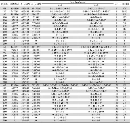
The results for instance Pn6k2-DS16N are presented in Table 3, considering different values of battery

autonomy Q and three values for parameter M described in equation (7). This parameter restricts the

number of arcs entering and leaving an EVCS, limiting indirectly the number of vehicles that can visit

the EVCS. For example, if M=1, one EV is allowed to visit the EVCS. If M=2, only two EVs are

permitted to enter an EVCS, and if M=150 (or a big number), all the EVs in the routing problem can visit

the EVCS.

Table 3

Results for instance Pn6k2-DS16N

Q [km] α [USD] β [USD] ω [USD] _k₌₁ Details of route _k₌₂ M Time [s]

65 154430 483983 3515056 0-5-22-19-1-20-4-0' 0-13-2-3-17-6-0' 1 809 80 247088 663491 4454116 0-11-14-3-6-2-12-0' 0-10-1-20-4-5-22-19-13-0' 1 1940 90 185316 600830 2862231 0-13-3-6-2-12-0' 0-11-1-20-4-5-19-10-0' 1 860

100 92658 423713 1355481 0-12-1-3-6-2-10-0' 0-5-20-4-0' 1 177 110 92658 450983 1112783 0-1-20-5-0' 0-4-19-3-6-2-10-0' 1 112

120 61772 419941 728485 0-2-6-3-20-4-0' 0-1-19-5-0' 1 70

130 61772 420425 728485 0-2-6-3-19-0' 0-1-20-4-5-0' 1 67

140 61772 413734 717722 0-4-19-5-0' 0-10-2-6-3-1-0' 1 114

150 61772 413734 717722 0-1-3-6-2-10-0' 0-5-19-4-0' 1 164

160 30886 356486 381939 0-4-5-0' 0-1-3-6-2-10-0' 1 10

170 30886 356486 381939 0-1-3-6-2-10-0' 0-4-5-0' 1 18

180 0 324905 0 0-5-4-0' 0-2-6-3-1-0' 1 5

200 0 324905 0 0-2-6-3-1-0' 0-5-4-0' 1 5

65 123544 566686 3171244 0-13-2-3-17-6-0' 0-13-17-1-20-22-5-22-20-4-0' 2 709

80 92658 571488 1355481 0-10-20-4-5-20-1-10-0' 0-12-3-6-2-12-0' 2 136 90 92658 571055 1355481 0-10-6-3-2-12-0' 0-12-1-20-5-4-20-10-0' 2 403

100 61772 426025 773007 0-4-20-5-0' 0-1-20-3-6-2-10-0' 2 41 110 61772 426025 773007 0-1-20-5-0' 0-10-2-6-3-20-4-0' 2 149

120 30886 394444 388708 0-4-20-5-0' 0-1-20-3-6-2-0' 2 31

130 30886 394444 388708 0-1-20-5-0' 0-4-20-3-6-2-0' 2 40

140 30886 394444 388708 0-1-20-3-6-2-0' 0-4-20-5-0' 2 47

150 30886 394444 388708 0-4-20-3-6-2-0' 0-1-20-5-0' 2 23

160 30886 356486 381939 0-5-4-0' 0-10-2-6-3-1-0' 2 19

170 30886 356486 381939 0-4-5-0' 0-1-3-6-2-10-0' 2 18

180 0 324905 0 0-1-3-6-2-0' 0-4-5-0' 2 5

200 0 324905 0 0-5-4-0' 0-1-3-6-2-0' 2 5

65 123544 649628 2133795 0-13-12-20-22-5-22-4-20-12-13-0' 0-13-12-1-20-3-6-2-12-13-0' 150 109 80 61772 542047 968403 0-12-20-4-5-20-1-12-0' 0-12-3-6-2-12-0' 150 54 90 61772 542047 968403 0-12-2-6-3-12-0' 0-12-1-20-4-5-20-0' 150 112

100 30886 449419 388708 0-20-3-6-2-1-20-0' 0-5-20-4-0' 150 28 110 30886 449419 388708 0-20-3-6-2-1-20-0' 0-4-20-5-0' 150 29

120 30886 394444 388708 0-2-6-3-20-1-0' 0-4-20-5-0' 150 21

130 30886 394444 388708 0-2-6-3-20-4-0' 0-5-20-1-0' 150 24

140 30886 394444 388708 0-4-20-5-0' 0-1-20-3-6-2-0' 150 33

150 30886 394444 388708 0-2-6-3-20-4-0' 0-1-20-5-0' 150 27

160 30886 356486 381939 0-4-5-0' 0-1-3-6-2-10-0' 150 13

170 30886 356486 381939 0-10-2-6-3-1-0' 0-4-5-0' 150 20

180 0 324905 0 0-1-3-6-2-0' 0-5-4-0' 150 3

200 0 324905 0 0-1-3-6-2-0' 0-4-5-0' 150 3

According to Table 3, as the battery autonomy (first column) is increased for a certain value of M (column

7), there is a reduction of the cost associated with EVCS installation, EVs routing and PDS energy losses (second, third and fourth columns respectively). Columns 5 and 6 show the nodes sequence traveled by

the EVs, with the EVCSs identified in bold. When the battery autonomy Q is large enough (Q>180 km),

no EVCSs are installed and the terms α and ω are zero, obtaining the same results as those presented in

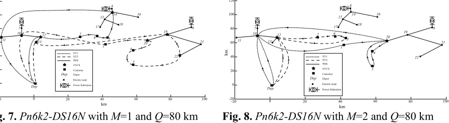
benchmark case. Fig. 7 depicts the EVs routes and the EVCSs installed along the PDS for instance

(12)

visiting EVCS in 11, EV1 has to visit another EVCS located at node 14, as the recharge acquired in 11

is not sufficient to visit all customers and come back to the depot. For values of Q greater or equal than

80 km, the third term γ of the objective function is always zero. For values of Q less than 80 km, i.e.,

Q=65 km in Table 3, the term γ is greater than zero. This situation suggests an upgrade in the battery,

because along the routes, the autonomy for both EVs is not sufficient to complete some arcs and installing

more EVCSs could incur in a relevant increase of energy losses (installation of EVCSs at nodes quite far

from the substation). Specifically, for Q=65 km and M=150, the route traveled by EV1 is the longest path

found in all the runs shown in Table 3. Due to M has a big number, there are more options to go back to

depot after visiting customers and the routing length becomes longer than other cases. In contrast with

this case, the routing length is smaller for Q=65 km and M=1, as the EVCS revisit is not permitted,

reducing the options for EVs to go back to depot.

Fig. 7.Pn6k2-DS16N with M=1 and Q=80 km Fig. 8.Pn6k2-DS16N with M=2 and Q=80 km

For M=2 and Q=80 km, the graphic result is shown in Fig. 8. Due to M=2, the number of arcs entering

and leaving an EVCS installed can be less or equal than 2. Even if M=2 some of the EVCSs receive one

vehicle, which visits the EVCS, then goes to visit other customers and come back to the same EVCS to recharge the battery and continue with the travel. This case applies for EV2, which once leaves from node 12 (EVCS installed), visits the customers at nodes 3, 6 and 2, and returns to node 12. The same situation happens for EV1, when revisits EVCS installed at node 20 after visiting customers at nodes 4

and 5. When M=150 and Q=80 km, the behavior is pretty the same as that presented in Fig. 8. While

for M=2, EV1 visits the EVCS installed at node 10, the routing sequence (see this case in Table 3) changes

slightly when M=150, as EV1 visits EVCS at node 12 (which is also visited by EV2). This is the result

of relaxing the parameter M with a big number, allowing the EVCS to receive several EVs. In this sense,

the number of EVCSs is reduced, resulting in the decrease of energy losses in PDS.

4.2. Pn7k3-DS34N

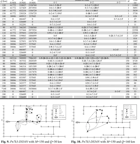
Following the same dynamic with Pn6k2-DS16N, the results for Pn7k3-DS34N are presented in Table 4.

In this latter, the execution time increases compared with Pn6k2-DS16N for the majority of the cases,

because the introduction of more customers and vehicles (since the transportation approach), and the enlargement of the PDS contributes to a greater degree of the computational effort. In some cases all the

three vehicles are used. For those runs where Q<120 km, Q<90 km and Q<30 km for M=1, M=2 and

M=150 respectively, the solver failed and was not able to find a feasible solution after too long.

Considering the situation in which M=150 and Q=30, the graphic solution is depicted in Fig. 9. It is noted

from this case that the EVCSs are installed as closest as possible to the power substation located at node 8, as a measure to reduce energy losses. By the other side, the revisit is done in all the ECVSs installed,

due to relaxation of constraint in Eq. (7) by increasing parameter M.

Dep

9 10

15

11

16 14

6 7

2

4 1

3

5 12

13

17

19

20 18

21 8

120 100

80 60

40 20 0

-20

-20 0 20 40 60 80 100

22

km

Dep

EV1 EV2 PDS EVCS Customer Depot

Power Substation Electric node

Dep

9 10

15

11

16 14

6 7

2

4 1

3

5 12

13

17

19 20 18

21 8

120 100

80

60

40

20

0

-20

-20 0 20 40 60 80 100

22

km

Dep

(13)

A. Arias et al.

Table 4

Q [km] α [USD]

β

[USD]

ω

[USD]

Details of route _M Time [s]

k=1 k=2 k=3

120 61772 338027 2194760 0-6-1-5-21-0' 0-2-4-7-3-22-0' 1 11882

130 61772 327429 2073954 0-6-1-5-10-0' 0-3-7-4-2-20-0' 1 5691 140 61772 432216 1556729 0-3-7-9-2-4-0' 0-6-1-5-10-0' 1 5839

150 61772 330324 1556729 0-2-4-7-3-9-0' 0-10-5-1-6-0' 1 5730 160 30886 449912 537845 0-6-0' 0-2-4-7-3-9-0' 0-5-1-0' 1 626

170 0 466447 0 0-6-1-5-0' 0-3-0' 0-7-4-2-0' 1 27 180 0 326609 0 0-3-7-4-2-0' 0-6-1-5-0' 1 39

200 0 352291 0 0-7-3-2-4-0' 0-6-1-5-0' 1 11

90 61772 346245 2106560 0-10-6-1-5-21-0' 0-21-3-7-4-2-10-0' 2 32122

100 61772 337444 2073954 0-10-6-1-5-10-0' 0-20-2-4-7-3-20-0' 2 22598 110 61772 397053 1556729 0-9-3-7-4-2-10-0' 0-9-5-1-10-6-0' 2 27553

120 30886 339063 1084099 0-0' 0-6-1-5-21-0' 0-21-3-7-4-2-0' 2 1329 130 30886 329757 1051509 0-3-7-4-2-20-0' 0-6-1-5-20-0' 2 818

140 30886 327851 1017078 0-6-1-5-10-0' 0-3-7-4-2-10-0' 2 1002 150 30886 343577 537845 0-6-1-5-9-0' 0-2-4-7-3-9-0' 2 299

160 30886 343577 537845 0-9-3-7-4-2-0' 0-6-1-5-9-0' 2 103 170 0 466447 0 0-7-4-2-0' 0-5-1-6-0' 0-3-0' 2 82

180 0 326609 0 0-2-4-7-3-0' 0-5-1-6-0' 2 27

200 0 326609 0 0-0' 0-6-1-5-0' 0-3-7-4-2-0' 2 29 30 185316 509999 7986105 0-9-20-11-6-12-1-12-5-12-11-20-9- 0-9-20-22-2-22-3-23-4-23-7-22-20-9- 150 28010

60 61772 367532 2820349 0-11-5-1-6-11-0' 0-21-7-4-2-21-3-21-0' 150 6728 80 30886 426192 1084099 0-21-1-5-21-6-21-0' 0-21-2-4-7-3-21-0' 150 2683

90 30886 346314 1051509 0-20-2-4-7-3-20-0' 0-20-5-1-6-20-0' 150 411 100 30886 339333 1017078 0-10-6-1-5-10-0' 0-10-3-7-4-2-10-0' 150 1825

110 30886 339333 1017078 0-10-5-1-6-10-0' 0-10-2-4-7-3-10-0' 150 197 120 30886 339333 1017078 0-10-6-1-5-10-0' 0-10-2-4-7-3-10-0' 150 562

130 30886 453507 537845 0-9-2-4-7-3-9-0' 0-9-1-5-9-6-0' 150 177 140 30886 373938 537845 0-9-3-7-4-2-9-0' 0-9-6-1-5-9-0' 150 194

150 30886 343577 537845 0-6-1-5-9-0' 0-9-3-7-4-2-0' 150 88 160 30886 343577 537845 0-6-1-5-9-0' 0-2-4-7-3-9-0' 150 61

*160 30886 505182 3438866 0-3-7-4-35-1-0' 0-6-35-5-2-0' 150 9112 170 0 466447 0 0-6-1-5-0' 0-7-4-2-0' 0-3-0' 150 53

180 0 326609 0 0-5-1-6-0' 0-2-4-7-3-0' 150 35 200 0 326609 0 0-5-1-6-0' 0-2-4-7-3-0' 150 16

Note from Table 4 that this run has the longest computational time (around 8 hours) to obtain a solution, because the autonomy is slightly bigger than the distance between the depot and the closest electric node

where an EVCS should be installed (dist(Dep-9)=29.33 km). This fact contributes that finding a feasible

solution be hard as the battery autonomy is barely enough to complete the route. Looking into a larger

autonomy, Fig. 10 represents the solution with M=150 and Q=160. In this situation, the behavior is

consistent in regards the location of the EVCS close to the power substation (at node 9). See that only one EVCS is installed to virtually increase the battery autonomy and meet the customers. However, other situations should be studied, for example: Fig. 11 shows that a large portion of the nodes (area shaded) belonging PDS are not allowed to install EVCSs (nodes from 9 to15 and from 20 to 30) due to other issues (limitations associated with terrain topology, public space, right of way, etc.) that are not addressed in this work. In this sense, the EVCS should be installed at the node where the energy losses be as reduced

80 70 60 50 40 30 20 10 0 -10

-20_-40 _-20 ₀ ₂₀ ₄₀ ₆₀ ₈₀ ₁₀₀ ₁₂₀ ₁₄₀

4 5 6 7 14 15 16 17 20 21 22 23 36 37 38 39 40 18 19

8 9 10

35 13 12 2 3 1 11 41 Dep 30 31 32 33 34 25 26 24 27 28 29 km km Dep EV1 EV2 PDS EVCS Customer Depot Power Substation Electric node 80 70 60 50 40 30 20 10 0 -10

-20_-40 _-20 ₀ ₂₀ ₄₀ ₆₀ ₈₀ ₁₀₀ ₁₂₀ ₁₄₀

4 5 6 7 14 15 16 17 20 21 22 23 36 37 38 39 40 18 19

8 9 10

(14)

as possible. The solution shows that this can be reached by installing the EVCS at node 35, which is the next node out of the restricted area and with a less distance to the substation, compared with nodes 31,

32, 33 and 34. The costs and sequence of routes obtained for this solution are found in Table 4 at Q=*160

km.

Fig. 11.Pn7k3-DS34N with M=150 and Q=160 km, restricting EVCSs at nodes 9-15 and 20-30

4.3. Pn8k3-DS23N

As mentioned before, the addition of a new customer to the transportation network, contributes to

increase computational effort for finding a solution, which can be seen in Table 5 for instance

Pn8k3-DS23N.

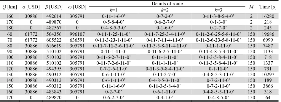
Table 5

Q [km] α [USD] β [USD] ω [USD] Details of route M Time [s]

k=1 k=2 k=3

160 30886 492614 305791 0-11-1-6-0’ 0-7-2-0’ 0-11-3-8-5-4-0’ 2 16280

170 0 489870 0 0-5-8-4-0’ 0-6-2-7-0’ 0-1-3-0’ 2 218

180 0 482567 0 0-4-8-5-3-0’ 0-1-6-0’ 0-2-7-0’ 2 245

60 61772 564356 996107 0-11-1-25-11-0’ 0-11-7-25-3-4-11-0’ 0-11-2-6-25-5-8-11-0’ 150 19686

70 61772 605522 636591 0-11-3-23-1-11-0’ 0-11-7-11-4-11-0’ 0-11-2-6-23-5-8-11-0’ 150 6999

80 30886 616619 305791 0-11-7-11-2-6-11-0’ 0-11-3-5-8-11-4-11-0’ 0-11-1-11-0’ 150 7487

90 30886 510102 305791 0-11-1-11-0’ 0-11-6-2-7-11-0’ 0-11-4-8-5-3-11-0’ 150 1133

100 30886 510102 305791 0-11-6-2-7-11-0’ 0-11-1-11-0’ 0-11-3-5-8-4-11-0’ 150 718

110 30886 510102 305791 0-11-7-2-6-11-0’ 0-11-1-11-0’ 0-11-3-5-8-4-11-0’ 150 1337

120 30886 494395 305791 0-7-2-6-11-0’ 0-11-3-5-8-4-11-0’ 0-1-11-0’ 150 791

130 30886 490312 305791 0-6-1-11-0’ 0-11-2-7-0’ 0-4-8-5-3-11-0’ 150 10297

140 30886 490312 305791 0-6-1-11-0’ 0-4-8-5-3-11-0’ 0-7-2-11-0’ 150 189

150 30886 490312 305791 0-11-1-6-0’ 0-11-3-5-8-4-0’ 0-7-2-11-0’ 150 3866

160 30886 483843 305791 0-2-7-0’ 0-6-1-11-0’ 0-4-8-5-3-11-0’ 150 318

170 0 489870 0 0-6-2-7-0’ 0-3-1-0’ 0-4-8-5-0’ 150 64

Even if the mathematical model is relaxed with M=150 for constraint in (7), run time is notably long

compared with the instances Pn6k2-DS16Nand Pn7k3-DS34Nfor similar cases of battery autonomy Q.

It is not possible for solver to find a solution for cases when M=1 (not presented in Table 5) and the

installation of EVCSs is required, i.e., when the solution is different from the benchmark case. By the

other side, when M=2 and Q<160 km no solution is found, because the number of customers and

limitation in parameter M (which greatly restricts the mathematical model) makes impossible to get at

least a feasible solution, due to an exact solution technique is being used. Routing solution with M=2 and

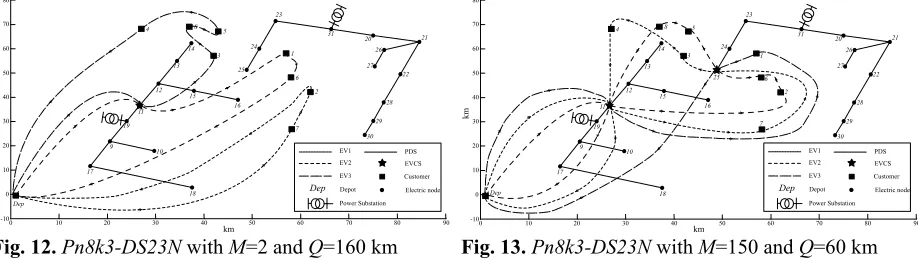
Q=160 km is shown in Fig. 12. See that Q is barely sufficient to complete a big portion of the routes

length, being necessary the installation of only one EVCS for EV2 and EV3. EV1 is able to meet its respective customers with autonomy assigned.

80 70 60 50 40 30 20 10 0 -10 -20

-40 -20 0 20 40 60 80 100 120 140

4

5

6 7

14 15

16

17

20 21 22 23

36 37

38 39 40

18

19

8 9 10

35

13 12 2

3

1

11

41 Dep

30 31 32

33

34

25

26

24 27 28 29

km

Dep

(15)

A. Arias et al.

In contrast with case mentioned above, Fig. 13 illustrates a different situation in which M is increased

(relaxed mathematical model) and autonomy is reduced. For M=150 and Q=60 km, the installation of

two EVCSs is required at both feeders of the PDS. According to Table 5, it is worth to mention that in this case the cost for energy losses is increased in three times compared with situation shown in Fig. 12. Likewise, it is noted that both EVCSs are visited by all EVs to renew autonomy and meet customers.

5. Conclusions

This paper presented an electric vehicle integrated planning problem (EVs-IPP) model to improve the performance of transportation network and power distribution system PDS. A sensitivity analysis was performed by relaxing mathematical model and using different values of EVs’ battery autonomy. In this manner, the number of EVs permitted to be recharged at a given EVCS was under control, examining different costs for each solution, i.e., EVCSs installed along the PDS, EVs routing and energy losses. The cases in which was not necessary to install EVCSs due to the high battery autonomy, the results related with routing (transportation network approach) and power flow (PDS approach) were quite similar to those obtained in the benchmark case. By restricting some nodes at the PDS, EVCSs were located as closest as possible to the power feeder substation, in order to make minimum the energy losses. The latter greatly contribute to objective function when the EVCSs are subjected to receive only one

vehicle. In the cases, where a comparison with autonomy could be done, i.e., for Pn6k2-DS16N instance

with M=1, the energy losses cost was 16 times greater than those presented when the EVCSs are able to

receive all the EVs (M=150). Due to the existence of several terms in objective function, the problem

could be treated since the point of view of the multi-objective optimization. By varying weighting factors, a set of solutions can be built up, represented along a Pareto front. However, the proposed model can be solved by using meta-heuristic techniques such as NSGA II, SPEA, Epsilon Constraint, among others, to find a front of solutions with different weights for each objective. In this work, concrete values for weighting factors in the objective function were used, in order to represent consistently the priorities established by the decision maker, which would be the owner of both, the transportation and power distribution networks. Otherwise, the problem should be dealt as a bi-level problem, where the solution of the routing and EVCSs installation costs would be the input to find the energy losses on the power flow formulation.

References

Agenbroad, J. (2014). Pulling Back the Veil on EV Charging Station Costs - Rocky Mountain Institute. Rocky Mountain Institute. https://www.rmi.org/news/pulling-back-veil-ev-charging-station-costs/ (June 1, 2017). Arias, A., Martínez, L. H., Hincapie, R. A., & Granada, M. (2015, October). An IEEE Xplore database literature

review regarding the interaction between electric vehicles and power grids. In Innovative Smart Grid

Technologies Latin America (ISGT LATAM), 2015 IEEE PES (pp. 673-678). IEEE.

Chan, C. C. (1999). The past, present and future of electric vehicle development. In Power Electronics and Drive

Systems, 1999. PEDS'99. Proceedings of the IEEE 1999 International Conference on (Vol. 1, pp. 11-13). IEEE.

Christofides, N., Mingozzi, A., & Toth, P. (1977). The vehicle routing problem. In Combinatorial Optimization,

Dep 80 70 60 50 40 30 20 10 0

-10₀ ₁₀ ₂₀ ₃₀ ₄₀ ₅₀ ₆₀ ₇₀ ₈₀ ₉₀

1 6 2 7 3 5 8 4 9 10 11 12 14 15 16 17 18 19 13 28 20 21 23 24 25 29 27 22 26 30 31 km km Dep EV1 EV2 PDS EVCS Customer Depot Power Substation Electric node EV3 Dep 80 70 60 50 40 30 20 10 0

-10₀ ₁₀ ₂₀ ₃₀ ₄₀ ₅₀ ₆₀ ₇₀ ₈₀ ₉₀

(16)

Society for Industrial and Applied Mathematics, 315–38.

Civanlar, S., Grainger, J. J., Yin, H., & Lee, S. S. H. (1988). Distribution feeder reconfiguration for loss reduction. IEEE Transactions on Power Delivery, 3(3), 1217-1223.

Dong, X., Mu, Y., Jia, H., Wu, J., & Yu, X. (2016). Planning of fast EV charging stations on a round freeway. IEEE Transactions on Sustainable Energy, 7(4), 1452-1461.

Du, Y., Zhou, X., Bai, S., Lukic, S., & Huang, A. (2010, February). Review of non-isolated bi-directional DC-DC converters for plug-in hybrid electric vehicle charge station application at municipal parking decks. In Applied

Power Electronics Conference and Exposition (APEC), 2010 Twenty-Fifth Annual IEEE (pp. 1145-1151).

IEEE.

GAMS Development Corporation. (2016). GAMS Solvers. https://gams.com/latest/docs/solvers/index.html (June 1, 2017).

Hannan, M. A., Lipu, M. S. H., Hussain, A., & Mohamed, A. (2017). A review of lithium-ion battery state of charge estimation and management system in electric vehicle applications: Challenges and recommendations. Renewable and Sustainable Energy Reviews, 78, 834-854.

Intergovernmental Panel on Climate Change. (2015). Climate change 2014: mitigation of climate change (Vol. 3). Cambridge University Press.

Liu, Z. F., Zhang, W., Ji, X., & Li, K. (2012, May). Optimal planning of charging station for electric vehicle based on particle swarm optimization. In Innovative Smart Grid Technologies-Asia (ISGT Asia), 2012 IEEE (pp. 1-5). IEEE.

Luo, C., Huang, Y. F., & Gupta, V. (2017). Placement of EV Charging Stations—Balancing Benefits Among Multiple Entities. IEEE Transactions on Smart Grid, 8(2), 759-768.

Miranda, V., Ranito, J. V., & Proenca, L. M. (1994). Genetic algorithms in optimal multistage distribution network planning. IEEE Transactions on Power Systems, 9(4), 1927-1933.

Mock, P. (2014). EU CO2 standards for passenger cars and light-commercial vehicles. The International Council

on Clear Transportation.

NEO Networking and Emerging Optimization. (2013). VRP Instances: Vehicle Routing Problem. http://neo.lcc.uma.es/vrp/vrp-instances/ (June 1, 2017).

Neyestani, N., Damavandi, M. Y., Shafie-Khah, M., Contreras, J., & Catalão, J. P. (2015). Allocation of plug-in vehicles' parking lots in distribution systems considering network-constrained objectives. IEEE Transactions on Power Systems, 30(5), 2643-2656.

Pazouki, S., Mohsenzadeh, A., Ardalan, S., & Haghifam, M. R. (2015). Simultaneous planning of PEV charging stations and DGs considering financial, technical, and environmental effects. Canadian Journal of Electrical

and Computer Engineering, 38(3), 238-245.

Power Systems Planning Group. (2017). Electric Vehicles Integrated Planning Problem Test Systems. http://academia.utp.edu.co/planeamiento/sistemas-de-prueba/evs-ipp/ (June 2, 2017).

Ribeiro, É. T. A. (2013). Modelos de programação inteira mista para a alocação ótima de bancos de capacitores em sistemas de distribuição de energia elétrica radias.

Shojaabadi, S., Abapour, S., Abapour, M., & Nahavandi, A. (2016). Optimal planning of plug-in hybrid electric vehicle charging station in distribution network considering demand response programs and uncertainties. IET Generation, Transmission & Distribution, 10(13), 3330-3340.

Tanaka, N. (2011). Technology roadmap: Electric and plug-in hybrid electric vehicles. International Energy Agency, Tech. Rep.

Tesla Supercharger. (2017). https://www.tesla.com/supercharger (June 1, 2017).

U.S. Department of Energy. (2017). Alternative Fuels Data Center: Charging Plug-In Electric Vehicles at Home.” Energy Efficiency & Renewable Energy. https://www.afdc.energy.gov/fuels/electricity_charging_home.html (June 1, 2017).

Worley, O., Klabjan, D., & Sweda, T. M. (2012, March). Simultaneous vehicle routing and charging station siting for commercial electric vehicles. In Electric Vehicle Conference (IEVC), 2012 IEEE International (pp. 1-3). IEEE.

Yang, J., & Sun, H. (2015). Battery swap station location-routing problem with capacitated electric vehicles. Computers & Operations Research, 55, 217-232.