Sensitivity to Prior Specification in
Bayesian Identification of Autoregressive Time Series Models
Ayman A Amin
Department of Statistics, Mathematics and Insurance Faculty of Commerce, Menoufia University, Egypt [email protected]
Abstract
In this paper we use the Kullback-Leibler divergence to measure the distance between the posteriors of autoregressive (AR) model order, aiming to evaluate mathematically the sensitivity of the model identification to different types of priors of the model parameters. In particular, we consider three priors for the AR model coefficients, namely Jeffreys', g, and natural conjugate priors, and three priors for the model order including uniform, arithmetic, and geometric priors. Using a large number of Monte Carlo simulations with various values of the model coefficients, model order, and sample size, we evaluate the impact of the posteriors distance in the accuracy of the model identification. Simulation study results show that the posterior of the model order is sensitive to prior distributions, and the highest accuracy of the model identification is obtained from the posterior resulting from the g-prior. Same results are obtained from the application to real-world time series datasets.
Keywords: Distance of posteriors, Kullback-Leibler divergence, Jeffreys’ prior, g-prior, Natural conjugate prior.
1. Introduction
Prior specification plays an important role in the Bayesian analysis of time series models. This is because the posterior density of the model parameters is obtained by combining the prior distribution of these parameters with the likelihood function of the observed time series (Broemeling, 1985). Different types of prior distributions are employed in the Bayesian time series analysis to represent the information about the parameters of time series model. Schlaifer and Raiffa (1961) presented a natural conjugate prior that has a distributional form depends on the likelihood function form to guarantee obtaining an analytically tractable posterior distribution. In case of little or no information is available about the model parameters, Jeffreys (1961) introduced a prior, known as Jeffreys’ proir, which overcomes the lack of invariance property of other existing non-informative priors. In order to simplify the elicitation of covariances of the model parameters, Zellner (1986) presented a reference informative prior known as g-prior. The availability of different types of priors makes the prior selection a complicated task and raises the issue of model identification sensitivity to prior distributions.
(Fan and Yao, 2009), multivariate autoregressive models (Shaarawy and Ali, 2008), and multivariate moving average models (Shaarawy and Ali, 2012). These researchers have employed one or more of the abovementioned prior distributions to derive the posterior mass function of the model order, however, none of them has evaluated the sensitivity of model identification to different types of prior distributions. Recently, Soliman et al. (2015) have tried to evaluate the sensitivity of model identification to prior selection, however, their work is only based on empirical results and depends on a small scale of simulation study. Therefore, there is a need in the Bayesian time series analysis for a comprehensive and sophisticated evaluation of the model identification sensitivity to different priors to help researchers in the phase of prior specification.
In this paper, we use the Kullback-Leibler (KL) divergence (Kullback and Leibler, 1951) to measure the distance between the posteriors of the AR model order, resulting from different types of priors, in order to evaluate mathematically the sensitivity of the model identification to the employed priors. In addition, we evaluate the impact of the posteriors distance in the accuracy of model identification using a large number of Monte Carlo simulations. Accordingly, our work in this paper can be summarized in the following. First, we consider three types of priors for the AR model coefficient, namely Jeffreys’, g, and natural conjugate priors, and also three priors for the AR model order including uniform, arithmetic, and geometric priors in order to obtain the posterior mass functions of the AR model order. Second, we compute the KL divergence and its calibration between the resulting posteriors to measure the distance between these posteriors. Third, we execute a large number of Monte Carlo simulations with various values of the model coefficients, model order, and sample size in order to evaluate the impact of the posteriors distance in the accuracy of model identification. Finally, we use real-world time series datasets to illustrate the use of the KL divergence to measure the distance between the posteriors and show the impact of this distance in the model identification.
The remainder of this paper is organized as follows. In Section 2 we present the background of the autoregressive time series model and its Bayesian concepts, and we obtain the marginal posteriors of the AR model order. In Section 3 we introduce the KL divergence and its calibration between the model order posteriors. In Section 4 we present simulation study and real-world time series datasets to illustrate the use of the KL divergence to measure the distance between the posteriors and then evaluate the impact of this distance in the model identification. Finally, we give the conclusions in Section 5.
2. Autoregressive Time Series Models and Bayesian Concepts
Time series {𝑦𝑡} can be modeled by an autoregressive (AR) model of order 𝑝, simply denoted by AR(𝑝), and written as (Box et al., 2015):
𝜙𝑝(𝐵)𝑦𝑡 = 𝜀𝑡 (1)
where {𝜀𝑡} is a sequence of independent and normally distributed errors with zero mean and variance 𝜎2, B is the backshift operator defined as 𝐵𝑑𝑥𝑡= 𝑥𝑡−𝑑, and 𝜙𝑝(𝐵) is the autoregressive polynomial with order 𝑝 written as 𝜙𝑝(𝐵) = (1 − 𝜙1𝐵 − ⋯ − 𝜙𝑝𝐵𝑝). The model (1) can be simplified and written as
where 𝑦 = (𝑦1, 𝑦2, ⋯ , 𝑦𝑛)𝑇, 𝑋 is an 𝑛 × 𝑝 design matrix with the 𝑡𝑡ℎ row 𝑋𝑡 =
(𝑦𝑡−1, … , 𝑦𝑡−𝑝), 𝜙 = (𝜙1, 𝜙2, … , 𝜙𝑝)𝑇 is the autoregressive coefficients, and 𝜀 =
(𝜀1, 𝜀2, … , 𝜀𝑛)𝑇.
It is worth noting that the design matrix 𝑋 becomes a function of 𝑝 when the AR model order is unknown. In this case we can assume that the model order 𝑝 is a random variable with a known maximum value of 𝑘. The prior information about 𝑝 can be represented in terms of a prior mass function 𝜁(𝑝) that can have different forms such as uniform, i.e.
𝜁(𝑝) = 1/𝑘, or geometric, i.e. 𝜁(𝑝) = 0. 5𝑝∀𝑝 = 1,2, . . . , 𝑘.
As we discussed above, we consider in this work three types of priors for the parameters
𝜙 and 𝜎2: natural conjugate prior, g-prior, and Jeffreys’ prior. The natural conjugate prior in the case of AR models with normally distributed errors is a normal-gamma distribution. Suppose 𝜙~𝑁𝑝(𝜇𝜙, 𝜎2Σ𝜙) and 𝜎2~𝐼𝐺(𝜈2,𝜆2), the joint natural conjugate prior distribution of 𝜙 and 𝜎2 is given by:
𝜁𝑛(𝜙, 𝜎2) ∝ (𝜎2)−(𝜈+𝑝2 +1)exp {− 1
2𝜎2[𝜆 + (𝜙 − 𝜇𝜙)
𝑇
Σ𝜙−1(𝜙 − 𝜇
𝜙)]}, (3) where 𝜇𝜙, Σ𝜙, 𝜈 and 𝜆 are hyperparameters need to be estimated.
The g-prior of 𝜙 and 𝜎2 can be written as:
𝜁𝑔(𝜙, 𝜎2) ∝ (𝜎2)−(𝑝2+1)exp {− 𝑔
2𝜎2(𝜙 − 𝜙̅)𝑇(𝑋𝑇𝑋)(𝜙 − 𝜙̅)}, (4)
where 𝜙̅ is an anticipated value of 𝜙, and g is a parameter that usually specified as a decreasing function of 𝑛 and 𝑝 (Fernandez et al., 2001).
Jeffreys’ prior of 𝜙 and 𝜎2 is given by:
𝜁𝑗(𝜙, 𝜎2) ∝ (𝜎2)−1, 𝜎2 > 0 (5)
The likelihood function of the AR model (2) can be obtained by employing a straightforward random variable transformation from 𝜀 to 𝑦, and written as
𝐿(𝜙, 𝜎2, 𝑝|𝑦) ∝ (𝜎2)−𝑛2exp {− 1
2𝜎2𝜀𝑇𝜀},
∝ (𝜎2)−𝑛2exp {− 1
2𝜎2(𝑦 − 𝑋𝜙)𝑇(𝑦 − 𝑋𝜙)}, (6)
Based on the likelihood function (6), we update the information about the AR model order 𝑝 by the posterior probability mass function. To derive this posterior mass function of 𝑝, we need first to obtain the joint posterior of the model parameters 𝜙, 𝜎2 and 𝑝, and then integrate out the parameters 𝜙 and 𝜎2.
We obtain the joint posterior of the parameters 𝜙, 𝜎2 and 𝑝 by multiplying the likelihood function by the joint prior of these parameters. For the natural conjugate prior, the joint posterior of 𝜙, 𝜎2 and 𝑝 is obtained as:
𝜁𝑛(𝜙, 𝜎2, 𝑝|𝑦) ∝ 𝜁(𝑝)(𝜎2)−(𝑛+𝜈+𝑝2 +1)exp {− 1
2𝜎2[𝜆 + (𝜙 − 𝜇𝜙) 𝑇
Σ𝜙−1(𝜙 − 𝜇 𝜙) +
We integrate out the parameters 𝜙 and 𝜎2 in (7) and obtain the marginal posterior mass function of the model order 𝑝 as:
𝜁𝑛(𝑝|𝑦) ∝ 𝜁(𝑝) [|Σ𝜙 −1| |𝐴𝑛|] 1 2 [𝑦𝑇𝑦 + 𝜆 + 𝜇
𝜙𝑇Σ𝜙−1𝜇𝜙− 𝐵𝑛𝑇𝐴−1𝑛 𝐵𝑛] −𝑛+𝜈2
∀𝑝 = 1,2, . . . , 𝑘.
Where 𝐴𝑛 = (𝑋𝑇𝑋 + Σ𝜙−1) and 𝐵𝑛 = (𝑋𝑇𝑦 + Σ𝜙−1𝜇𝜙)
For the g-prior, we obtain the joint posterior of 𝜙, 𝜎2 and 𝑝 as:
𝜁𝑔(𝜙, 𝜎2, 𝑝|𝑦) ∝ 𝜁(𝑝)(𝜎2)−(𝑛+𝑝2 +1)exp {− 1
2𝜎2[(𝜙 − 𝜙̅)𝑇(𝑔𝑋𝑇𝑋)(𝜙 − 𝜙̅) +
(𝑦 − 𝑋𝜙)𝑇(𝑦 − 𝑋𝜙)]}. (8)
By integrating out the parameters 𝜙 and 𝜎2 in (8), we obtain the marginal posterior mass function of 𝑝 as:
𝜁𝑔(𝑝|𝑦) ∝ 𝜁(𝑝) [𝑔 + 1𝑔 ]−
𝑛−𝑝 2
[𝑦𝑇𝑦 + 𝑔𝜙̅𝑇(𝑋𝑇𝑋)𝜙̅ − 𝐵
𝑔𝑇𝐴𝑔−1𝐵𝑔] −𝑛2
∀𝑝 = 1,2, . . . , 𝑘.
where 𝐴𝑔 = ((𝑔 + 1)𝑋𝑇𝑋) and 𝐵𝑔 = (𝑋𝑇𝑦 + 𝑔(𝑋𝑇𝑋)𝜙̅)
For Jeffreys’ prior, the joint posterior of 𝜙, 𝜎2 and 𝑝 is given by :
𝜁𝑗(𝜙, 𝜎2, 𝑝|𝑦) ∝ 𝜁(𝑝)(𝜎2)−(𝑛2+1)exp {− 1
2𝜎2(𝑦 − 𝑋𝜙)𝑇(𝑦 − 𝑋𝜙)}, (9)
Integrating out the parameters 𝜙 and 𝜎2 in (9) results in the marginal posterior mass function of 𝑝 as:
𝜁𝑗(𝑝|𝑦) ∝ 𝜁(𝑝) Γ (
𝑛−𝑝 2 )
𝜋𝑛−𝑝2 |𝑋𝑇𝑋| 1 2
[𝑦𝑇𝑦 − 𝑦𝑇𝑋(𝑋𝑇𝑋)−1𝑋𝑇𝑦]−𝑛−𝑝2 ∀𝑝 = 1,2, . . . , 𝑘.
3. Kullback-Leibler Divergence Between Posterior Mass Functions of Model Order
The distance between two probability mass functions, say 𝜁1(𝑥) and 𝜁2(𝑥), can be measured by the Kullback-Leibler (KL) divergence (Kullback and Leibler, 1951) defined as
𝐾𝐿[𝜁1(𝑥), 𝜁2(𝑥)] = 𝐸𝜁1(𝑥)[𝑙𝑛 (𝜁1(𝑥) 𝜁2(𝑥))],
= ∑𝑥 𝜁1(𝑥)𝑙𝑛 (𝜁𝜁1(𝑥)
2(𝑥)). (10)
The KL divergence between two posterior mass functions of 𝑝, say 𝜁1(𝑝|𝑦) and 𝜁2(𝑝|𝑦), can be computed as:
𝐾𝐿[𝜁1(𝑝|𝑦), 𝜁2(𝑝|𝑦)] = ∑𝑘𝑝=1𝜁1(𝑝|𝑦)𝑙𝑛 (𝜁𝜁1(𝑝|𝑦)
2(𝑝|𝑦)), (11)
and simplified to be:
𝐾𝐿[𝜁1(𝑝|𝑦), 𝜁2(𝑝|𝑦)] = ∑
𝑘
𝑝=1
𝜁1(𝑝|𝑦)[−𝑙𝑛(𝜁2(𝑝|𝑦))] − ∑
𝑘
𝑝=1
𝜁1(𝑝|𝑦)[−𝑙𝑛(𝜁1(𝑝|𝑦))],
= 𝐶𝐻[𝜁1(𝑝|𝑦), 𝜁2(𝑝|𝑦)] − 𝐻[𝜁1(𝑝|𝑦)], (12)
where the components 𝐶𝐻[𝜁1(𝑝|𝑦), (𝜁2(𝑝|𝑦)] and 𝐻[𝜁1(𝑝|𝑦)] are known as the cross-entropy and Shannon cross-entropy respectively. The KL divergence in (12) is asymmetric measure since it does not satisfy the triangle inequality (Contreras-Reyes and Arellano-Valle, 2012). However, we can get a symmetric distance by computing the average of two KL divergences as:
𝐾𝐿∗[𝜁
1(𝑝|𝑦), 𝜁2(𝑝|𝑦)] =
1
2{𝐾𝐿[𝜁1(𝑝|𝑦), 𝜁2(𝑝|𝑦)] + 𝐾𝐿[𝜁2(𝑝|𝑦), 𝜁1(𝑝|𝑦)]}
Values of the KL divergence are between 0 and ∞, and it can be calibrated to be between 0.5 and 1.0 to be easy to judge about the distance between the posteriors. Accordingly, when the calibration value of the KL divergence between two posteriors is close to 0.5, it implies the two posteriors are very similar; and when the value is close to 1.0 the two posteriors are strongly different and the prior specification is important in this case. Suppose 𝐾𝐿[𝜁1(𝜙|𝑦), 𝜁2(𝜙|𝑦)] = 𝛾, McCulloch (1989) proposed that the calibration of the KL divergence can be computed to be the value 𝛿 such that 𝐾𝐿[𝐵(0.5), 𝐵(𝛿)] = 𝛾, where 𝐵(𝛿) is a Bernoulli distribution with success probability 𝛿. Using the result that
𝐾𝐿[𝐵(0.5), 𝐵(𝛿)] = −𝑙𝑜𝑔(4𝛿(1 − 𝛿))/2 (McCulloch, 1989, Abramowitz and Stegun, 1972), we can compute the calibration of KL divergence (KLC) between two posteriors as:
𝐾𝐿𝐶[𝜁1(𝜙|𝑦), 𝜁2(𝜙|𝑦)] = 12{1 − 𝑒𝑥𝑝(−2𝐾𝐿[𝜁1(𝜙|𝑦), 𝜁2(𝜙|𝑦)])} (13)
The KL divergence in (12) and its calibration in (13) can be directly computed for any two of the marginal posteriors of 𝑝 presented in Section (2), and in the following section we evaluate these measures using simulated and real-world time series datasets.
4. Application
In this section we have two parts. In the first part, we present a simulation study to evaluate the KL divergence (and its calibration) between the posterior mass functions of the AR model order and evaluate its impact in the model identification. We present two applications of our work to real world time series datasets in the second part.
4.1Simulation Study
identification. We generate several time series data with considering different sample size, different model orders, and different values of the model coefficients.
For the prior specification in this simulation study, we employ the uniform prior for the model order 𝑝 with a known maximum 𝑘 = 4. In addition, we use three values for the parameter 𝑔, i.e. 1/𝑛, 𝑝/𝑛, and 𝑘𝑝/𝑛, for the g-prior, following the recommendations of Fernandez et al. (2001), and also we follow the training sample approach to estimate the hyperparamters of the natural conjugate prior (Berger, 1985, Rachev et al., 2008). To run the simulations, we generate 1,000 time series of size 𝑛 (from 50 to 400 with an increment of 50 observations) from AR models with orders 1 (𝜙 = 0.3, 0.5, and 0.8), 2 (𝜙1 = 0.5 and 0.2, and 𝜙2 = 0.4 and 0.6), and 3 (𝜙1 = 0.5 and 0.2, 𝜙2 = 0.4 and 0.6, and
𝜙3 = 0.4 and 0.6). For each time series, we compute the posterior mass functions of 𝑝,
𝜁𝑗(𝑝|𝑦), 𝜁𝑔(𝑝|𝑦), and 𝜁𝑛(𝑝|𝑦) resulting from the employed priors Jeffreys’, g, and natural conjugate respectively. Based on the computed posterior mass functions of 𝑝, we compute the KL divergence (and its calibration) between these posteriors, and identify the model order as a value with a maximum posterior probability. For all simulated time series, we compute the percentage of correctly identified models by comparing the identified order with the true value of 𝑝 used to generate the time series.
We present the average of KL divergence and its calibration obtained with the 1,000 time series for AR(1) with 𝜙 = 0.3 in Table (1) and particularly the boxplot of the KL calibration (for 𝑛 = 200) in Figure (1), and present the percentage of correctly identified models in Table (2). From these results, we observe that the KL divergence and its calibration between 𝜁𝑗(𝑝|𝑦) and 𝜁𝑔1(𝑝|𝑦) and those between 𝜁𝑗(𝑝|𝑦) and 𝜁𝑔3(𝑝|𝑦) are very close, for example when 𝑛 = 200 their calibration values are about 0.73. These divergences are strongly larger than those between 𝜁𝑗(𝑝|𝑦) and 𝜁𝑔2(𝑝|𝑦) and those between 𝜁𝑗(𝑝|𝑦) and 𝜁𝑛(𝑝|𝑦), which both have calibration values of about 0.6 for 𝑛 =
200 as an example. The impact of these posteriors divergences can be observed in the percentage of correctly identified models presented in Table (1), since the results show that the highest percentage of correctly identified models is obtained from the two posteriors resulting from the g-prior with 𝑔 = 1/𝑛 and 𝑘𝑝/𝑛 followed by the percentage obtained from the two posteriors resulting from the g-prior with 𝑔 = 𝑝/𝑛 and from the natural conjugate prior, and the lowest percentage is obtained from the posterior resulting from the Jeffreys’ prior. It is worth observing that when the sample size grows the divergences of posteriors mass functions are reduced. For large sample size (𝑛 = 400), all the KL calibration values are less than 0.7, and all the percentages of correctly identified models are greater than 95%. This confirms that the impact of the prior distribution will be eliminated for a large sample of observations.
Table 1: KL divergence and its calibration for AR(1) with 𝝓 = 𝟎. 𝟑
Sample size (𝒏)
50 100 150 200 250 300 350 400
𝑲𝑳[𝜻𝒋, 𝜻𝒈𝟏] ∗
0.322 0.211 0.164 0.134 0.122 0.109 0.101 0.093
𝑲𝑳𝑪[𝜻𝒋, 𝜻𝒈𝟏] 0.837 0.784 0.755 0.734 0.723 0.711 0.704 0.696
𝑲𝑳[𝜻𝒋, 𝜻𝒈𝟐] 0.068 0.038 0.028 0.023 0.021 0.019 0.016 0.015
𝑲𝑳𝑪[𝜻𝒋, 𝜻𝒈𝟐] 0.655 0.619 0.603 0.594 0.589 0.584 0.58 0.577
𝑲𝑳[𝜻𝒋, 𝜻𝒈𝟑] 0.315 0.207 0.161 0.13 0.119 0.106 0.099 0.091
𝑲𝑳𝑪[𝜻𝒋, 𝜻𝒈𝟑] 0.833 0.78 0.751 0.73 0.719 0.708 0.7 0.693
𝑲𝑳[𝜻𝒋, 𝜻𝒏] 0.112 0.067 0.052 0.039 0.037 0.032 0.029 0.026
𝑲𝑳𝑪[𝜻𝒋, 𝜻𝒏] 0.667 0.631 0.615 0.604 0.599 0.593 0.589 0.585
𝑲𝑳[𝜻𝒈𝟏, 𝜻𝒏] 0.19 0.147 0.126 0.107 0.1 0.09 0.085 0.081
𝑲𝑳𝑪[𝜻𝒈𝟏, 𝜻𝒏] 0.754 0.728 0.711 0.697 0.69 0.681 0.675 0.67
∗𝜁
𝑔1, 𝜁𝑔2, and 𝜁𝑔3 posteriors from g-prior with 𝑔 = 1/𝑛, 𝑝/𝑛 and 𝑘𝑝/𝑛 respectively, and 𝜁𝑗 and 𝜁𝑛 posteriors from Jeffreys’ and natural conjugate priors respectively.
Table 2: Percentage of correctly identified models for AR(1) with 𝝓 = 𝟎. 𝟑.
Sample size (𝒏)
50 100 150 200 250 300 350 400
𝜻𝒋(𝒑|𝒚) 76.6 87.2 90.8 92.9 92.9 95 94.9 95.8
𝜻𝒈𝟏(𝒑|𝒚) 93.9 97.1 97.9 98.4 98.6 98.6 97.8 98.3
𝜻𝒈𝟐(𝒑|𝒚) 87.2 92.5 94.7 95.2 94.9 96.6 96.3 97.2
𝜻𝒈𝟑(𝒑|𝒚) 94.3 96.8 98 98.3 98.3 98.5 97.8 98.3
Figure 1: Boxplot of the KL calibration for AR(1) with ϕ=0.3 and n=200
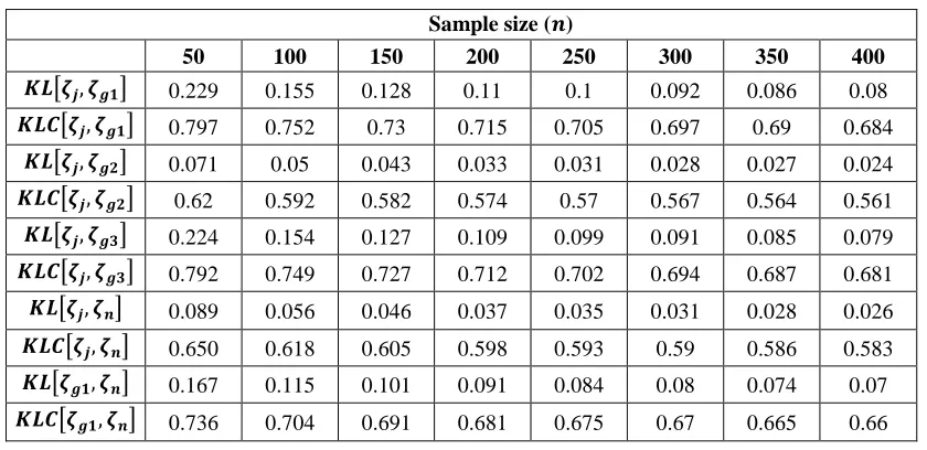
Table 3: KL divergence and its calibration for AR(2) with 𝝓𝟏= 𝟎. 𝟐 and 𝝓𝟐= 𝟎. 𝟔
Sample size (𝒏)
50 100 150 200 250 300 350 400
𝑲𝑳[𝜻𝒋, 𝜻𝒈𝟏] 0.229 0.155 0.128 0.11 0.1 0.092 0.086 0.08
𝑲𝑳𝑪[𝜻𝒋, 𝜻𝒈𝟏] 0.797 0.752 0.73 0.715 0.705 0.697 0.69 0.684
𝑲𝑳[𝜻𝒋, 𝜻𝒈𝟐] 0.071 0.05 0.043 0.033 0.031 0.028 0.027 0.024
𝑲𝑳𝑪[𝜻𝒋, 𝜻𝒈𝟐] 0.62 0.592 0.582 0.574 0.57 0.567 0.564 0.561
𝑲𝑳[𝜻𝒋, 𝜻𝒈𝟑] 0.224 0.154 0.127 0.109 0.099 0.091 0.085 0.079
𝑲𝑳𝑪[𝜻𝒋, 𝜻𝒈𝟑] 0.792 0.749 0.727 0.712 0.702 0.694 0.687 0.681
𝑲𝑳[𝜻𝒋, 𝜻𝒏] 0.089 0.056 0.046 0.037 0.035 0.031 0.028 0.026
𝑲𝑳𝑪[𝜻𝒋, 𝜻𝒏] 0.650 0.618 0.605 0.598 0.593 0.59 0.586 0.583
𝑲𝑳[𝜻𝒈𝟏, 𝜻𝒏] 0.167 0.115 0.101 0.091 0.084 0.08 0.074 0.07
𝑲𝑳𝑪[𝜻𝒈𝟏, 𝜻𝒏] 0.736 0.704 0.691 0.681 0.675 0.67 0.665 0.66
Table 4: Percentage of correctly identified models for AR(2) with 𝝓𝟏= 𝟎. 𝟐 and
𝝓𝟐= 𝟎. 𝟔.
Sample size (𝒏)
50 100 150 200 250 300 350 400
𝜻𝒋(𝒑|𝒚) 80.4 88.9 91.9 94.5 93.8 94.6 94.3 95.3
𝜻𝒈𝟏(𝒑|𝒚) 90.6 97.4 97.4 98.3 97.8 98.7 98.4 98.9
𝜻𝒈𝟐(𝒑|𝒚) 85.7 91.6 94.1 95 95.1 95.8 95.1 95.6
𝜻𝒈𝟑(𝒑|𝒚) 91.4 97.2 97.1 98.3 97.6 98.7 98.2 98.9
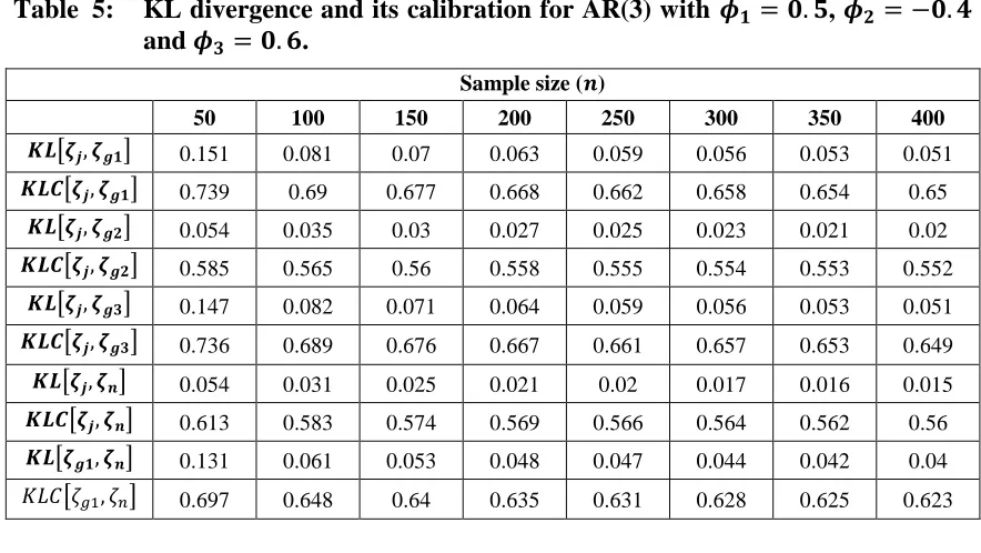
Table 5: KL divergence and its calibration for AR(3) with 𝝓𝟏= 𝟎. 𝟓, 𝝓𝟐= −𝟎. 𝟒 and 𝝓𝟑= 𝟎. 𝟔.
Sample size (𝒏)
50 100 150 200 250 300 350 400
𝑲𝑳[𝜻𝒋, 𝜻𝒈𝟏] 0.151 0.081 0.07 0.063 0.059 0.056 0.053 0.051
𝑲𝑳𝑪[𝜻𝒋, 𝜻𝒈𝟏] 0.739 0.69 0.677 0.668 0.662 0.658 0.654 0.65
𝑲𝑳[𝜻𝒋, 𝜻𝒈𝟐] 0.054 0.035 0.03 0.027 0.025 0.023 0.021 0.02
𝑲𝑳𝑪[𝜻𝒋, 𝜻𝒈𝟐] 0.585 0.565 0.56 0.558 0.555 0.554 0.553 0.552
𝑲𝑳[𝜻𝒋, 𝜻𝒈𝟑] 0.147 0.082 0.071 0.064 0.059 0.056 0.053 0.051
𝑲𝑳𝑪[𝜻𝒋, 𝜻𝒈𝟑] 0.736 0.689 0.676 0.667 0.661 0.657 0.653 0.649
𝑲𝑳[𝜻𝒋, 𝜻𝒏] 0.054 0.031 0.025 0.021 0.02 0.017 0.016 0.015
𝑲𝑳𝑪[𝜻𝒋, 𝜻𝒏] 0.613 0.583 0.574 0.569 0.566 0.564 0.562 0.56
𝑲𝑳[𝜻𝒈𝟏, 𝜻𝒏] 0.131 0.061 0.053 0.048 0.047 0.044 0.042 0.04
𝐾𝐿𝐶[𝜁𝑔1, 𝜁𝑛] 0.697 0.648 0.64 0.635 0.631 0.628 0.625 0.623
Table 6: Percentage of correctly identified models for AR(3) with 𝝓𝟏 = 𝟎. 𝟓, 𝝓𝟐 =
−𝟎. 𝟒 and 𝝓𝟑 = 𝟎. 𝟔.
Sample size (𝒏)
50 100 150 200 250 300 350 400
𝜻𝒋(𝒑|𝒚) 84.7 89.4 91.7 94.5 94.2 95.3 95.8 95.6
𝜻𝒈𝟏(𝒑|𝒚) 89.6 97.2 98.0 98.3 98.4 99.1 98.7 99.1
𝜻𝒈𝟐(𝒑|𝒚) 86.8 91.6 93.3 95.4 94.8 95.5 95.6 96.1
𝜻𝒈𝟑(𝒑|𝒚) 90.3 97.1 98.1 98.3 98.3 98.9 98.5 99.0
𝜻𝒏(𝒑|𝒚) 89.1 92.4 93.9 95.9 95.7 96.2 96.1 96.6
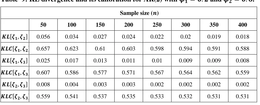
Now, one question can be raised: is there an impact for the prior distribution of the model order in the posteriors divergence and the percentage of correctly identified models? To answer this question we modify the simulation design to employ only the g-prior with
𝑔 = 1/𝑛 for the coefficients 𝜙, and employ three prior distributions for 𝑝 given as:
𝜁1(𝑝) =
1
𝑘, ∀𝑝 = 1,2, . . . , 𝑘 (Uniform prior) 𝜁2(𝑝) = 0. 5𝑝, ∀𝑝 = 1,2, . . . , 𝑘 (Geometric prior)
𝜁3(𝑝) =𝑘−𝑝+1𝑘+1 , ∀𝑝 = 1,2, . . . , 𝑘 (Arithmetic prior) (14)
In general, all simulation results show that the employed priors for the model order result in very similar posteriors. However, the posteriors of the model order resulting from the employed priors for the model coefficients are strongly different, and the highest percentage of identified models is obtained from the posterior resulting from the g-prior distribution.
Table 7: KL divergence and its calibration for AR(1) with 𝝓 = 𝟎. 𝟑
Sample size (𝒏)
50 100 150 200 250 300 350 400
𝑲𝑳[𝜻𝟏, 𝜻𝟐]∗ 0.059 0.04 0.032 0.026 0.024 0.021 0.02 0.018
𝑲𝑳𝑪[𝜻𝟏, 𝜻𝟐] 0.66 0.632 0.618 0.607 0.602 0.596 0.593 0.59
𝑲𝑳[𝜻𝟏, 𝜻𝟑] 0.019 0.012 0.009 0.007 0.006 0.005 0.005 0.005
𝑲𝑳𝑪[𝜻𝟏, 𝜻𝟑] 0.59 0.57 0.561 0.555 0.552 0.548 0.547 0.545
𝑲𝑳[𝜻𝟐, 𝜻𝟑] 0.013 0.009 0.008 0.007 0.006 0.005 0.005 0.005
𝑲𝑳𝑪[𝜻𝟐, 𝜻𝟑] 0.577 0.565 0.56 0.555 0.552 0.549 0.548 0.546 ∗𝜁
1, 𝜁2, and 𝜁3 are posteriors from priors 𝜁1(𝑝), 𝜁2(𝑝), and 𝜁3(𝑝), respectively.
Table 8: Percentage of correctly identified models for AR(1) with 𝝓 = 𝟎. 𝟑 .
Sample size (𝒏)
50 100 150 200 250 300 350 400
𝜻𝟏(𝒑|𝒚) 93.9 97.1 97.9 98.4 98.6 98.6 97.8 98.3
𝜻𝟐(𝒑|𝒚) 97.6 98.9 99.2 99.5 99.5 99.1 98.9 99.1
𝜻𝟑(𝒑|𝒚) 96.1 98.3 98.9 99.2 99 98.9 98.6 98.5
Table 9: KL divergence and its calibration for AR(2) with 𝝓𝟏 = 𝟎. 𝟐 and 𝝓𝟐 = 𝟎. 𝟔.
Sample size (𝒏)
50 100 150 200 250 300 350 400
𝑲𝑳[𝜻𝟏, 𝜻𝟐] 0.056 0.034 0.027 0.024 0.022 0.02 0.019 0.018
𝑲𝑳𝑪[𝜻𝟏, 𝜻𝟐] 0.657 0.623 0.61 0.603 0.598 0.594 0.591 0.588
𝑲𝑳[𝜻𝟏, 𝜻𝟑] 0.025 0.017 0.013 0.011 0.01 0.009 0.009 0.008
𝑲𝑳𝑪[𝜻𝟏, 𝜻𝟑] 0.607 0.586 0.577 0.571 0.567 0.564 0.562 0.559
𝑲𝑳[𝜻𝟐, 𝜻𝟑] 0.008 0.004 0.003 0.003 0.002 0.002 0.002 0.002
Table 10: Percentage of correctly identified models for AR(2) with 𝝓𝟏 = 𝟎. 𝟐 and
𝝓𝟐 = 𝟎. 𝟔.
Sample size (𝒏)
50 100 150 200 250 300 350 400
𝜻𝟏(𝒑|𝒚) 90.6 97.4 97.4 98.3 97.8 98.7 98.4 98.9
𝜻𝟐(𝒑|𝒚) 91.1 98.7 98.8 99.3 98.9 99.5 99.4 99.6
𝜻𝟑(𝒑|𝒚) 91.5 98.4 98.1 99.1 98.5 99.3 99.2 99.4
Table 11: KL divergence and its calibration for AR(3) with 𝝓𝟏= 𝟎. 𝟓, 𝝓𝟐= −𝟎. 𝟒 and 𝝓𝟑= 𝟎. 𝟔.
Sample size (𝒏)
50 100 150 200 250 300 350 400
𝑲𝑳[𝜻𝟏, 𝜻𝟐] 0.071 0.025 0.019 0.017 0.016 0.015 0.014 0.014
𝑲𝑳𝑪[𝜻𝟏, 𝜻𝟐] 0.662 0.605 0.595 0.589 0.586 0.583 0.581 0.578
𝑲𝑳[𝜻𝟏, 𝜻𝟑] 0.037 0.023 0.019 0.017 0.016 0.015 0.014 0.014
𝑲𝑳𝑪[𝜻𝟏, 𝜻𝟑] 0.629 0.603 0.595 0.589 0.586 0.583 0.581 0.578
𝑲𝑳[𝜻𝟐, 𝜻𝟑] 0.011 0.001 0.000 0.000 0.000 0.000 0.000 0.000
𝑲𝑳𝑪[𝜻𝟐, 𝜻𝟑] 0.549 0.504 0.500 0.500 0.500 0.500 0.500 0.500
Table 12: Percentage of correctly identified models for AR(3) with 𝝓𝟏= 𝟎. 𝟓,
𝝓𝟐 = −𝟎. 𝟒 and 𝝓𝟑= 𝟎. 𝟔.
Sample size (𝒏)
50 100 150 200 250 300 350 400
𝜻𝟏(𝒑|𝒚) 89.6 97.2 98 98.3 98.4 99.1 98.7 99.1
𝜻𝟐(𝒑|𝒚) 85.7 98 99.1 99.5 99.6 99.6 99.6 99.6
𝜻𝟑(𝒑|𝒚) 88.9 98.2 99.1 99.5 99.6 99.6 99.6 99.6
4.2Application to Real-World Time Series
Table 13: Description of the real-world time series datasets (Box et al., 2015)
Series Description Sample size
A Readings of chemical process temperature are collected every minute by temporarily disconnecting the controllers and recording the subsequent fluctuations in temperature.
226
B Readings of chemical process viscosity are collected every hour to show the effect of uncontrolled factors such as variations in ambient temperature.
310
C Numbers of annual Wolfer sunspot are collected over the period 1770 - 1869.
100
D Yields are collected from consecutive batches of a chemical process.
70
(a) Chemical process temperature readings (b) Chemical process viscosity readings
(c) Annual Wolfer sunspot numbers (d) Yields from chemical process batches
Using the non-Bayesian approach, Box et al. (2015) identified AR(1) model for the time series A and B, and identified AR(2) model for the time series C and D. We first employ Jeffreys’, g, and natural conjugate priors to obtain the posteriors of the model order. Second, we compute the KL divergence and its calibration between these posteriors. Finally, we compute the posterior probabilities and identify the model order with the maximum posterior probability. Results of the KL divergence and its calibration presented in Table (14) and results of the posterior probability and identified model are presented in Table (15). It can be observed that these results are very consistent with the results from the simulation study in previous subsection, and the identified models are almost the same as those identified by the non-Bayesian approach.
Table 14: KL divergence and its calibration for the real-world datasets.
Real-world time series
A B C D
𝑲𝑳[𝜻𝒋, 𝜻𝒈𝟏] 0.081 0.175 0.269 0.358
𝑲𝑳𝑪[𝜻𝒋, 𝜻𝒈𝟏] 0.693 0.772 0.823 0.858
𝑲𝑳[𝜻𝒋, 𝜻𝒈𝟐] 0.007 0.05 0.001 0.06
𝑲𝑳𝑪[𝜻𝒋, 𝜻𝒈𝟐] 0.56 0.655 0.523 0.668
𝑲𝑳[𝜻𝒋, 𝜻𝒈𝟑] 0.077 0.155 0.258 0.357
𝑲𝑳𝑪[𝜻𝒋, 𝜻𝒈𝟑] 0.689 0.758 0.817 0.857
𝑲𝑳[𝜻𝒋, 𝜻𝒏] 0.005 0.045 0.012 0.12
𝑲𝑳𝑪[𝜻𝒋, 𝜻𝒏] 0.55 0.647 0.577 0.731
𝑲𝑳[𝜻𝒈𝟏, 𝜻𝒏] 0.06 0.091 0.169 0.069
𝑲𝑳𝑪[𝜻𝒈𝟏, 𝜻𝒏] 0.669 0.704 0.768 0.68
Table 15: Posterior probability and identified models for the real-world time series.
Series A Series B
𝒑 𝜻𝒋(𝒑|𝒚) 𝜻𝒈𝟏(𝒑|𝒚) 𝜻𝒈𝟐(𝒑|𝒚)𝜻𝒈𝟑(𝒑|𝒚) 𝜻𝒏(𝒑|𝒚) 𝜻𝒋(𝒑|𝒚) 𝜻𝒈𝟏(𝒑|𝒚) 𝜻𝒈𝟐(𝒑|𝒚) 𝜻𝒈𝟑(𝒑|𝒚) 𝜻𝒏(𝒑|𝒚)
1 0.811 0.929 0.853 0.925 0.821 0.811 0.881 0.789 0.865 0.719
2 0.143 0.065 0.117 0.069 0.151 0.143 0.105 0.168 0.120 0.228
3 0.032 0.005 0.02 0.005 0.021 0.032 0.010 0.029 0.011 0.043
4 0.014 0.001 0.01 0.001 0.007 0.014 0.003 0.014 0.004 0.009
Identified 𝒑 AR(1) AR(1) AR(1) AR(1) AR(1) AR(1) AR(1) AR(1) AR(1) AR(1)
Series C Series D
𝒑 𝜻𝒋(𝒑|𝒚) 𝜻𝒈𝟏(𝒑|𝒚) 𝜻𝒈𝟐(𝒑|𝒚)𝜻𝒈𝟑(𝒑|𝒚) 𝜻𝒏(𝒑|𝒚) 𝜻𝒋(𝒑|𝒚) 𝜻𝒈𝟏(𝒑|𝒚) 𝜻𝒈𝟐(𝒑|𝒚) 𝜻𝒈𝟑(𝒑|𝒚) 𝜻𝒏(𝒑|𝒚)
1 0.000 0.001 0.000 0.001 0.000 0.067 0.268 0.127 0.27 0.146
2 0.477 0.797 0.489 0.79 0.544 0.318 0.464 0.382 0.458 0.449
3 0.18 0.114 0.163 0.116 0.181 0.443 0.24 0.409 0.244 0.341
4 0.343 0.089 0.348 0.092 0.275 0.172 0.028 0.082 0.028 0.064
5. Conclusions
In this paper we first obtained the posterior mass functions of the AR model order by considering three types of priors for the AR model coefficients, namely Jeffreys’, g, and natural conjugate priors, and three priors for the model order including uniform, arithmetic, and geometric priors. We then introduced the KL divergence and its calibration between the resulting posteriors to measure the distance between these posteriors. We used a large number of Monte Carlo simulations to evaluate the impact of the posteriors distance in the accuracy of model identification. Simulation results confirmed that the posteriors resulting from Jeffreys’, g, and natural conjugate priors are strongly different, and the highest percentage of identified models is obtained from employing the g-prior distribution. Along with the simulation study, we applied our work to real-world time series datasets and their results are consistent with those of the simulation study and the non-Bayesian approach. Future work may be an extension to multivariate autoregressive models.
References
1. Abramowitz, M., and Stegun, I. A. (1972). Handbook of mathematical functions with formulas, graphs, and mathematical table. Dover Publications, Inc.
2. Berger, J. (1985). Statistical decision theory and Bayesian analysis. Springer.
3. Box, G. E. P., Jenkins, G. M., Reinsel, G. C., and Ljung, G. M. (2015). Time Series Analysis: Forecasting and Control. John Wiley & Sons.
4. Broemeling, L. D. (1985). Bayesian analysis of linear models. CRC Press.
5. Contreras-Reyes, J. E., and Arellano-Valle R. B. (2012). Kullback-leibler divergence measure for multivariate skew-normal distributions. Entropy, 14(9): 1606-1626.
6. Diaz, J., and Farah, J. L. (1981). Bayesian identification of autoregressive process. In proceedings of the 22nd NBER-NSC Seminar on Bayesian Inference in Econo-metrics.
7. Fan, C., and Yao, S. (2009). Bayesian approach for arma process and its application. International Business Research, 1(4): 49-55.
8. Fernandez, C., Ley, E.. and Steel, M. F. (2001). Benchmark priors for bayesian model averaging. Journal of Econometrics, 100(2): 381-427.
9. Jeffreys, H. (1961). The theory of probability. Oxford University Press, London.
10. Kullback, S., and Leibler, R. A. (1951). On information and sufficiency. The annals of mathematical statistics, 22(1): 79-86.
11. McCulloch, R. E. (1989). Local model influence. Journal of the American Statistical Association, 84(406): 473-478.
12. Rachev, S. T., Hsu, J. S., Bagasheva, B. S., and Fabozzi, F. J. (2008). Bayesian methods in finance, volume 153. John Wiley & Sons.
14. Shaarawy, S. M., and Ali, S. S. (2008). Bayesian identification of multivariate autoregressive processes. Communications in Statistics - Theory and Methods, 37(5): 791- 802.
15. Shaarawy, S. M., and Ali, S. S. (2012). Bayesian model order selection of vector mov¬ing average processes. Communications in Statistics - Theory and Methods, 41(4): 684-698.
16. Shaarawy, S. M., Soliman, E. E. A., and Ali, S. S. (2007). Bayesian identification of moving average models. Communications in Statistics - Theory and Methods, 36(12): 2301-2312.
17. Soliman, E. E. A., Shaarawy, S. M., and Sorour, W. W. (2015). On bayesian identification of autoregressive processes. Pakistan Journal of Statistics and Operation Research, 11(1): 2301-2312.