IEEE802.11a Standard
Shaghayegh Kordnoori
Department of Statistics,
Science and Research Branch, Islamic Azad University, Tehran, Iran [email protected]
Hamidreza Mostafaei
Department of Statistics,
Tehran North Branch, Islamic Azad University, Tehran, Iran [email protected]
Mohammad Hassan Behzadi
Department of Statistics,
Science and Research Branch, Islamic Azad University, Iran [email protected]
Abstract
The Markov order is a crucial measure of the memory of a process and its information is essential for appropriate simulation of aspects of the process. In this paper, we suggest a robust and straightforward exact significance test based on generating surrogate data to assess the Markov order of a time series. This method is valid for any sample size and certifies a uniform sampling from the set of sequences that definitely have the nth order characteristics of the observed data. The Markov property and order of IEEE802.11a errors are investigated using this test.
Keywords: Markov order, Whittle's formula, Surrogate data, IEEE 802.11a
Introduction
In this paper, we first describe briefly the testing Markov order using the 𝜒2statistics for the large sample limit. Next, the exact significance test is explained according to surrogate data generation and Whittle's formula for any sample size. Finally, this exact significance test is applied for the error data of IEEE802.11a based OFDM system to test the Markov property and find the order of the Markov model.
The Mathematical Model
Markov Order Test for Large Sample
Suppose P be a 𝑁 × 𝑁 matrix with elements {𝑃𝑖𝑗: 𝑖, 𝑗 = 1, … , 𝑁} a random process
(𝑋0, 𝑋1, … ) with finite state space 𝑆 = {𝑠1, 𝑠2, … , 𝑠𝑁} is said to be a (homogenous)
Markov chain with transition matrix P if for all n,∀𝑖, 𝑗 ∈ {1, … , 𝑁} and ∀𝑖0, … , 𝑖𝑛−1 ∈
{1, … , 𝑁} we have Eq. 1:
𝑃(𝑋𝑛+1= 𝑆𝑗|𝑋0 = 𝑖0, 𝑋1 = 𝑖1, … , 𝑋𝑛−1 = 𝑖𝑛−1, 𝑋𝑛 = 𝑖)
= 𝑃(𝑋𝑛+1 = 𝑆𝑗|𝑋𝑛 = 𝑖) = 𝑃𝑖,𝑗 (1) Which implies that the future depends on the past only through the present and not on prior states.
Goodness-of-fit tests play a crucial role in applied and theoretical statistics. They are helpful in evaluating whether a statistical model is consistent with available data. The goodness-of-fit test for the Markov assumption is another pivotal issue. The exact goodness-of-fit tests for first and higher order Markov chains is presented in (Besag J., Mondal D., 2013) . Testing the Markov assumption is equivalent to test whether the sojourn time in each state follows an exponential distribution. Some usually applied methods testing whether random variables follow an exponential distribution are according to the empirical distribution function (EDF). Following the theory of (Billingsley, 1961) and the suggestions of (Hoel, 1954), we offer the following method for different types of modeling and testing Markov chains. Suppose 𝐸𝑤 be the expected frequency where ∑ 𝐸𝑤=N-2 and w indicate the set of all frequencies which the expected frequency is greater than zero; Furthermore, let 𝑂𝑤 ≥ 0 be the corresponding frequency
from the observed data. The asymptotic 𝜒2 test statistic is defined as Eq.2
𝜒2 = ∑(𝐸𝑤− 𝑂𝑤)2
𝐸𝑤 𝑤
(2)
Given the degrees of freedom d, The distribution 𝑓(𝜒2; 𝑑)is known when 𝑁 → ∞ and the p-value can be achieved by integrating 𝑓(𝜒2) over 𝜒2 ≥ 𝜒2𝑜𝑏𝑠. The degrees of freedom is considered as N(N-1).
Markov Order Test for any Sample Size
The described hypothesis test depends on the 𝜒2 distribution allowed in the asymptotic limit of infinite data, therefore it is not exact. Evaluating 𝜒2 for all admissible sequences that satisfy the null hypothesis is vital to find the exact distribution for finite data. Suppose a sequence of observations 𝒙 = {𝑥1, … , 𝑥𝑁} constitutes a Markov chain of order
that 𝛤(𝒙) indicate the set of sequences with the same F and the same beginning and end states as the observed sequence x.
The number of sequences with the word transition count F and start with state k and end with state l is determined by Whittle's formula, Eq.3:
𝑁𝑘𝑙(𝐹) = ∏ 𝐹𝑖 𝑖.!
∏ 𝐹𝑖,𝑗 𝑖𝑗!𝐶𝑘𝑙 (3)
Where 𝐹𝑖. is the sum of row i and 𝐶𝑘𝑙 is the (k,l)th cofactor of the matrix
𝐹𝑘𝑙∗ = { 𝑖𝑓 𝐹𝑖.=0
𝑖𝑓 𝐹𝑖.>0
𝛿𝑖𝑗
𝛿𝑖𝑗−𝐹𝑖𝑗⁄𝐹𝑖.
(4)
The value of (1) is so large that can not be calculated using fixed accuracy. Therefore, we instead calculate the algorithm of (3) applying a Stirling series for the factorial terms Eq.5:
ln 𝑥! ~𝑥𝑙𝑛 𝑥 − 𝑥 +12ln(2𝜋𝑥) +12𝑥1 −360𝑥1 3+1260𝑥1 5−1680𝑥1 7 (5) When 𝑥 > 16.
The fraction of sequences in 𝛤(𝒙) that have 𝜒2 values greater than or equal to 𝜒2𝑜𝑏𝑠 yields the p-value. The p-value can be estimated to any desired accuracy provided one has a technique of producing uniform random samples from the set 𝛤 even if |𝛤| is too large to enumerate all sequences. The previous techniques for generating samples from 𝛤 are not feasible, specifically for higher order testing. We give a practical method in the next part.
The Algorithm of Surrogate Generation
The Whittle formula is used for generating a sample subset of 𝛤 in a way that the sample is uniform. Given a transition matrix, a Whittle surrogate is a random sequence which is produced with exactly the same transition count and the beginning and end words are the same as the original sequence. This property assures that the transition probabilities are exactly the same as the original sequence. We consecutively extend a surrogate sequence, starting with a first state until all transitions are utilized. At each step the next state is selected according to the number of remaining sequences calculated by Whittle's formula, Moreover, in order to show the reduced transition count resulting from the selection, F is updated. The algorithm is certified to result in an acceptable surrogate since states are selected probabilistically weighted by the number of available sequences and the states that result in zero valid sequences are never selected.
Let the sequence 𝑧 = {𝑧1, … , 𝑧𝑁} be the member of 𝛤 beginning with 𝑧1 = 𝑘, ending with 𝑧𝑁 = 𝑙, and having the transition count matrix F. The nominees for the second element 𝑧2 are the set {𝑤|𝐹𝑧1𝑤>0}. For each nominee w we calculate 𝑁𝑤𝑙(𝐹′), the number of sequences left. Here 𝐹𝑖𝑗′ = 𝐹𝑖𝑗 − 𝛿𝑧1𝑤 is the original transition count matrix
minus the candidate transition. A nominee is chosen arbitrarily in proportion to the number of remaining sequences. Therefore
𝑃(𝑧2 = 𝑤) =𝑁𝑤𝑙(𝐹
′)
𝑁𝑧1𝑙(𝐹) (6)
alternative of 𝑧1 = 𝑧𝑁. For the case (𝑥1 ≠ 𝑥𝑁) then one must select 𝑧1 = 𝑥1 and 𝑧𝑁 =
𝑥𝑁. The advantages of this technique is its ability of generating long surrogates as the complication increases only linearly with N.
(Pethel S. D., Hahs D. W., 2014) proved that the surrogate data statistics behave as expected in the asymptotic limit even for a small sample and for this purpose, they computed the size and power of asymptotic and the exact 𝜒2 test for different orders of Markov processes using 2500 trials with 2500 surrogates. The p-value which is the fraction of these surrogate sequences that has 𝜒2 ≥ 𝜒2𝑜𝑏𝑠 was calculated.
The (n+1)th order entropy rate 𝐻𝑠𝑢𝑟𝑔which its computation is easier than the 𝜒2 test is an alternative statistic as follow Eq.7.:
𝐻(𝑥𝑡+1|𝑥𝑡, … , 𝑥𝑡−𝑛) = 𝐻(𝑥𝑡+1, 𝑥𝑡, … , 𝑥𝑡−𝑛) − 𝐻(𝑥𝑡, … , 𝑥𝑡−𝑛) (7)
A sequence of observations form a Markov chain of order n if
𝑃(𝑥𝑡+1|𝑥𝑡, 𝑥𝑡−1… ) = P(𝑥𝑡+1|𝑥𝑡, … , 𝑥𝑡−𝑛+1) (8)
or
𝐻(𝑥𝑡+1|𝑥𝑡, 𝑥𝑡−1… ) =H(𝑥𝑡+1|𝑥𝑡, … , 𝑥𝑡−𝑛+1) (9)
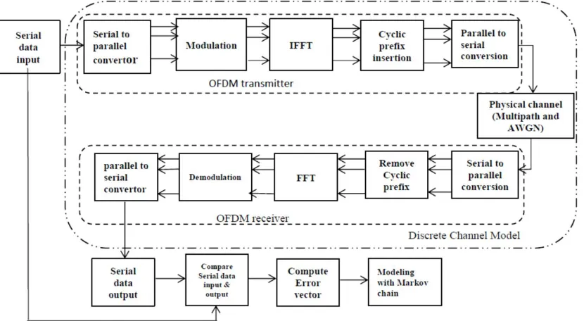
The Application of the Method
as a consequence of imperfections in the transmitter, channel and receiver is achieved by comparing the transmitted and received signal.
Figure 1: Block diagram for computing error vector and Markov modeling for OFDM.
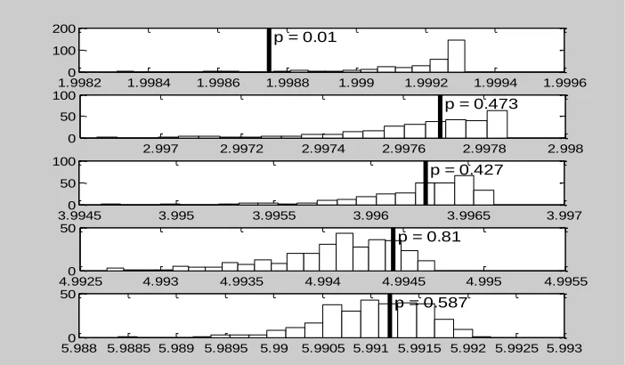
Figure 2: Block entropy histograms of the surrogate data for Markov orders zero through four, respectively. Solid vertical bars show the corresponding block entropy of the errors of the IEEE 802.11a OFDM system with 5200 binary error data and 400 surrogate data.
Figure 3: Block entropy histograms of the surrogate data for Markov orders zero through four, respectively. Solid vertical bars show the corresponding block entropy of the errors of the IEEE 802.11a OFDM system with 7280 binary error data and 300 surrogate data.
Conclusions
In this paper, we have explained the asymptotic chi square and new exact test of the null hypothesis that a Markov chain is from nth order. The exact test algorithm is more precise for small data than the asymptotic chi square test. This algorithm is according to
1.99840 1.9986 1.9988 1.999 1.9992 1.9994 1.9996 1.9998 2 200
400
p = 0.0375
2.9972 2.9974 2.9976 2.9978 2.998 2.9982 2.9984 2.9986 2.9988 0
50 100
p = 0.302
3.9950 3.9955 3.996 3.9965 3.997 3.9975 3.998 3.9985
50 100
p = 0.265
4.9905 4.991 4.9915 4.992 4.9925 4.993 4.9935 4.994 4.9945 4.995 4.99550 50
100
p = 0.875
5.9870 5.988 5.989 5.99 5.991 5.992 5.993 5.994
50 100
p = 0.2
1.99820 1.9984 1.9986 1.9988 1.999 1.9992 1.9994 1.9996
100 200
p = 0.01
2.997 2.9972 2.9974 2.9976 2.9978 2.998
0 50 100
p = 0.473
3.99450 3.995 3.9955 3.996 3.9965 3.997
50 100
p = 0.427
4.99250 4.993 4.9935 4.994 4.9945 4.995 4.9955
50
p = 0.81
5.988 5.9885 5.989 5.98950 5.99 5.9905 5.991 5.9915 5.992 5.9925 5.993 50
counts as the observed sequence. We have applied the Whittle's algorithm together with the entropy rate statistics for the IEEE802.11a (Wi-Fi) standard errors based on OFDM modulation to test the Markov property and the proper order. We have concluded that these errors have Markov property and their proper order is one. This approach is simple and there is no need for calculating the degrees of freedom or correcting for the small sample size.
References
1. Abdelrahman R. B. M., Mustafa A. B. A.,Osman A. A. (2015). A Comparison between IEEE 802.11a, b, g, n and ac Standards. IOSR Journal of Computer Engineering,17 (5,Ver. III), 26-29.
2. Baigorri A. R., Gonçalves C., Angelo P. (2009). Markov Chain Order Estimation and Relative Entropy. Retrieved from https://arxiv.org.
3. Besag J., Mondal D. (2013). Exact goodness-of-fit tests for Markov chains. Biometrics, 69(2), 488-96.
4. Billingsley, P. (1961). Statistical Methods in Markov Chains. Annals of Mathematical Statistics, 32(1), 12-40.
5. Bolch G., Greiner S., Meer H., Trivedi K. (2006). Queueing networks and Markov chains: modeling and performance evaluation with computer science applications. 2nd edition, John Wiley& Sons, Inc., publication.
6. Cinlar, E. (1975). Introduction to stochastic processes. Prentice-Hall, Englewood Cliffs, NJ.
7. Davis, J. C. (1973). Statistics and data analysis in geology.Wiley, New york,550p. 8. Deni, S. M., Jemain, A. A., Ibrahim K. (2009). Fitting optimum order of Markov chain models for daily rainfall occurrences in Peninsular Malaysia. Theoretical and Applied Climatology, 97, 109-121.
9. Ding J.,Tarokh V.,Yang Y. (2017). Bridging AIC and BIC: A New Criterion for Autoregression . IEEE TRANSACTIONS ON INFORMATION THEORY.
10. Dorea C. C. Y., Angelo P., Gonçalves C. (2015). Comparing the markov order estimators AIC, BIC and EDC . Transactions on Engineering Technologies, 41-54.
11. Feller, W. (1968). An introduction to probability theory and its applications. vol 1, John Wiley, New York, 3rd Edition.
12. Hlavičková I. (2015). An application of Markov chains in digital communication. Tatra Mountains Mathematical Publications, 63(1), 129-137.
13. Hoel, P. (1954). A Test for Markoff Chains (Vols. 41,Parts 3 and 4). Cambridge: University Press.
14. Howard, H. (1971). Dynamic probabilistic systems, Semi Markov and decision processes. John Wiley, New York, vol 2.
15. Huang J., Huang W., Chu P., Lee W., Pai H., Chuang C., Wu Y. (2017). Applying a Markov chain for the stock pricing of a novel forecasting model. Communications in Statistics-Theory and Methods, 46(9).
16. Ivan, B. (2015). Markov chain-like quantum biological modeling of mutations. aging and evolution, Life(Bsel), 5(3), 1518-1538.
18. Jónás T.,Kalló N., Eszter Tóth Z. (2014). Application of Markov Chains for Modeling and Managing Industrial Electronic Repair Processes. Periodica Polytechnica Social and Management Sciences,22(2), 87-98.
19. Katz, R. (1981). On some criteria for estimating the order of a Markov chain. TECHNOMETRICS, 23(3).
20. Krumbein, W. C.,Dacey, M. F. (1969). Markov chains and embedded Markov chains in geology. Jour. Internat. Assoc. Math. Geology, 1(1), 79–96.
21. Menendez M., Pardo L., Pardo M., Zografos K. (2011). Testing the order of Markov dependence in DNA sequences. Methodology and Computing in applied probability, 13, 59-74. 22. Merhav N., Gutman M., Ziv J. (1989). On the estimation of the order of a Markov chain and universal data compression . IEEE Transactions on Information Theory, 35(5), 1014 – 1019. 23. Mostafaei Hr., Kordnoori Sh., Kordnoori Sh. (2016). Using weighted Markov SCGM(1,1)c model to forecast gold/oil ,DJIA/gold and USD/XAU ratios. Malaysian Journal of fundamental and applied sciences, 12(4), 138-142.
24. Oviedo-Trespalacios O.,baena R. P., Mantilla M., Lacouture C. (2014). The Application of the Markov Chain in Statistical Quality Monitoring. Int'l Journal of Advances in Mechanical & Automobile Engg. (IJAMAE), 1(1), 68-72.
25. Papapetron M., Kugiumtzis D. (2016). Markov chain order estimation with parametric significance tests of conditional mutual information. Simulation modeling practice and theory, 61, 1-13.
26. Pardo, L. (2006). Statistical inference based on divergence measures. Chapman and Hall, New York.
27. Pethel S. D., Hahs D. W. (2014). Exact significance test for Markov order. Physica D, 269, 42-47.
28. Tamir, A. (1998). Applications of Markov Chains in Chemical Engineering. 1st Edition, Elsevier Science, 108-119.
29. Xianda C., Kyung T. K., Hee Y. Y. (2016). Integration of Markov random field with Markov chain for efficient event detection using wireless sensor network. Computer Network.