AB TEMPORAL TRIP GENERATION MODELLING FOR PRIMARY
ACTIVITIES: A CASE STUDY OF FAST GROWING METROPOLITAN CITY
Krishna Saw1, Bhimaji K. Katti2, Gaurang J. Joshi3
1, 2, 3 Civil Engineering Department,SVNIT, Surat, Gujarat-395007, India
Received 29 June 2014; accepted 21 January 2015
Abstract: Transportation planning for any city evolves on the basis of complex interplay between urban activity, transport and land use system to result in varied travel patterns. Travel pattern can be defined at micro level to include individual journey departure and arrival time, journey duration and distances to make way for temporal trip generation and distribution from specific area. Trip generation is the first step of four stages of travel forecasting analysis mostly followed all over the world. Traditionally, it is focused on the prediction of aggregate trip generation by a household rather than the choice of individual activity participation. However, spatial and temporal activity domains are equally important in forecasting process and strategic urban transportation planning. The present paper attempts to develop Activity Based (AB) Temporal Trip Generation Models (ABTGM) for primary activities to cover work and educational trips considering fast growing Surat city of Gujarat, India as study area. Home interview surveys are carried to provide household and socioeconomic characteristics and the activity travel diary information to focus on the activity based tours rather the trips. Keywords:activity system, travel pattern, temporal trip generation, activity.
1. Introduction
Trip generation is the first step of the four-step travel forecasting modelling procedure. It is a very important step since it sets up not only the framework for the subsequent forecasting tasks but also the magnitudes of zonal trip productions. But, this model explicitly ignores the spatial and temporal inter-connectivity inherent in household travel behavior (Jovicic, 2001; McNally and Rindt, 2007). The fundamental theory of travel demand, that travel is a demand derived from the demand for activity participation (Bowman, 1998), is explicitly ignored. The main limitations of the Four-Stage Model can be noted that the focus rest on trips for the purposes rather the tours with the sequence of activities, there by missing spatial and temporal considerations
(Ruey, 1997). The approach adopts a holistic framework that recognizes the complex interactions in activity and travel behaviour. Therefore, by predicting which activities are performed at particular destinations and times, trips and their timing and locations are implicitly forecasted in activity based model (Bhat and Singh, 2000).
2. Study Area: Brief
as ONGC, Reliance, ESSAR, and Shell are also in the vicinity. Having strong industrial base, urbanization of the city is of higher order to extent of 65%+ as decadal growth.
High rate of growth experienced by the city over five successive decades has been a significant feature urban growth dynamics (Table 1).
Table 1
Demographic Profile of Surat
Year 1961 1971 1981 1991 2001 2011
Population (lacs) 2.88 4.72 7.77 14.99 28.77 44.7
Decadal growth (%) 29.00 63.89 64.62 92.92 91.93 55.37
Source: Surat Municipal Corporation
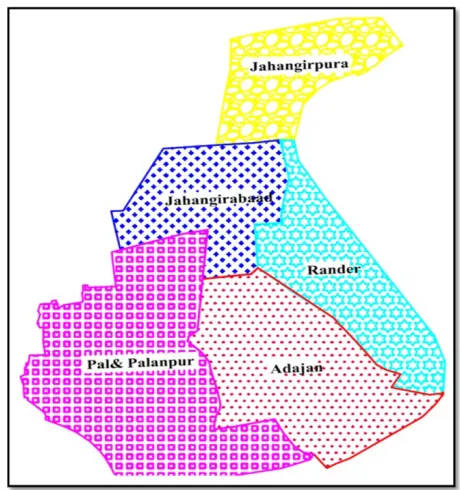
The number of vehicles in the city has gone up from 2.94 lacs in 1991 to 15.85 lacs in 2010 to reflect on urbanization impact. The city is spread over 326 sq. km with nearly 48 lacs populations to date. A part of the West Zone one of the seven administrative
zones of the city situated on left bank of river is the study area having nearly 4.05 lacs population covered over 28.68 sq. km area. The area is further divided in five sub zones (Fig. 1) with the particulars as shown in Table 2.
Table 2
Population and Household of West Zone (2011)
Sub-Zone Area (km2) Population No of Household
Adajan 6.73 196850 45993
Rander 5.12 114586 23290
Jahangirpura 3.616 27807 5584
Jahangirabad 4.16 6221 1567
Pal 6.045 36108 9118
Palan pur 3.008 23492 5932
Total 28.679 405064 85900
Source: Surat Municipal Corporation
3. Modelling Approach
3.1. Disaggregate Approach
The proposed approach is an activity-based modelling method which can be reduced to the conventional approach, thereby ensuring compatibility with the remainder of the four-step process. Basically it is disaggregated modelling approach requiring a comprehensive travel diary with detail activity information on activity scheduling and activity locations. The disaggregation is carried in two levels as household attributes and travel attributes. Ruey (1997) used disaggregate approach in his study. Due to the treatment of household variables used in the modelling process, the proposed trip generation model can estimate trip rates per household per day or per person per day. It is focused on personal tours rather than trips where tour is defined as chain of trips to start from home and ends at home. Bowman and Ben Akiva (2000) considered the daily activity travel pattern as set of tours in their study.
3.2. Primary, Secondary Tours and
Activities
Activities are prioritized on the basis of the purpose of activities. Work Activity
has been observed on priority followed by education and all other purposes. Activities with having higher duration can be assigned higher priorities. The tour of the day with highest priority or primary activities is designated the “primary” tour and others as secondary tours. The present work covers the primary tours of the day (Yagi and Mohammadian, 2010). Here the tour is used as unit of modelling travel instead of the trip preserving a consistency in destination, mode and time of day across the trips. Therefore the primary activities are first classified to realize daily activity patterns. Further the work related or other purpose trips if any are noted on en-route which may result into chain of trips.
3.3. Time of Day Choice
and Timmermans, 2011). The mode and destination choices are the other aspects that can be captured (Kitamura, 1996).
However, the proposed model is basically trip generation model and does not cover the mode and destination choices.
Table 3
Time Segmentation
Description Time Segmentation Remarks
Early Morning 6:00 - 9:00 Pre Peak
Morning 9:00 - 11:00 Peak Movements
Mid Day 11:00 - 14:00 Moderate
Early Evening 14:00 - 17:00 Off peak
Evening 17:00 - 20:00 Peak
Night 20:00 - 22:00 Off peak
Late Night 22:00+ Lean Period
3.4. Trip Transformation
It is required to reorient the tours to trips in the present trip generation model with reference to household members travel itinerary of the day. Three main categories such as Home Based Onward Trips (HBOT), Home Based Return Trips (HBRT), and Non-Home Based Trips (NHBT) can be identified from the tours. Secondary tours have the both home base and non home base trips. For example, going to the restaurant
from the work base non-home trip which is related to work related secondary tour.
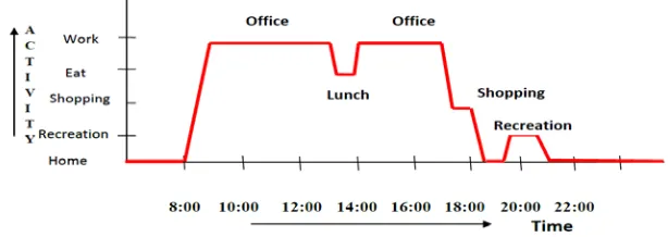
Ty pical Spatial and Temporal Tours presented in Fig. 2, to explain the tour and trip relations on time and activity axis, the inclined lines indicate the travel time function where as horizontals indicates activity time consumption. The sketch as such depicts the place of activities, time of activity and travel time as part of works diary itinerary.
Fig. 2.
Tour to trip transformation for the above itinerary is given below (Table 4).
Table 4
Tour to Trip Transformation
Type of Trip Primary Tour Pri-SubTour Secondary Tour
HBOT 1-Home to Office 1-Shopping 1-Going Recreation
HBRT 1-Return to home Nil 1-Return from Recreation
NHBT Nil 2-Lunch Nil
Total seven trips are performed. Here, the tours performed with in the primary tour are considered as Pri-Sub Tour.
4. Study Data Analysis
Home interviews surveys were carried employing the enumerators to collect the required information on household, socioeconomic characteristic and activity travel pattern particulars in all the five subzones as mentioned earlier. The household information is mainly on household size, age structure, family structure where as occupation, vehicle ownership and income pertain to socioeconomic characteristics. Activity and travel pattern are important segments of the activity travel pattern information (Bhat and Koppelman, 2003).
Here, information on life cycle, primary tours, secondary tours and discretionary tours play vital role in the analysis and building of the model where on activity duration for the various purposes, activity distance frequency and travel time frequency are important aspects in supporting of travel patterns. Secondary and discretionary tours are outside the scope of the present study. The base data required in the present study to build the AB base temporal trip generation model are only given below.
4.1. Household Structure and Trip Rates
Average household size and as well family structure in terms of working member and school and college going member etc. for the five sub-zones are shown in Table 5.
Table 5 Family Structure
Sub-Zone WM* SM* CM* Baby(<5)* NWM* HHS*
Adajan 1.44 0.72 0.44 0.23 1.44 4.28
Rander 1.63 0.84 0.54 0.21 1.7 4.92
Jahgirabaad (J. Baad) 1.46 0.71 0.6 0.12 1.08 3.97
Jahagirpura (J. Pura) 1.71 1.13 0.27 0.25 1.62 4.98
Pal+Palanpur (P+P) 1.33 0.8 0.3 0.24 1.28 3.96
The trip rates computation for the work and education purpose and total trips including other purposes per household are shown in Table
6. The variation in the data can be observed for the all five subzones owing to socioeconomic and land use characteristics prevailing.
Table 6
Work and Education Trip Rates
Sub-Zone Work-TPHD* Education-TPHD* Total-TPHD*
Adajan 3.07 2.53 7.84
Rander 2.78 2.67 7.43
J.Baad 3.38 3.28 9.17
J. Pura 3.65 3.59 9.75
P+P 3.11 2.95 8.11
West Zone 3.2 3 8.46
*TPHPD-Trip per Household per Day
4.2. Tour Categories
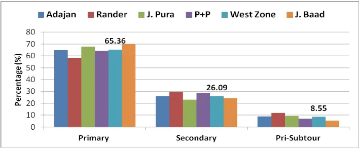
As the model associated with the tours, the observed data on primary, secondary and sub
tours are indicated in the following Fig. 3. Nearly 65% of the tours belong to primary and 26% to the secondary with marginal variations for the all subzones.
Fig. 3.
Tour Distribution of Subzone
4.3. Trip Distribution
Primary and secondary categories of trips are further grouped in terms of purposes as given below. Work and education trips are the major
Table 7
Purpose Wise Trip Distribution of Sub-Zones
Sub-Zone Work (%) Education (%) Shopping (%) Recreation (%) Other (%)
Adajan 40 25 14 10 11
Rander 33 25 12 17 13
J.Baad 38 32 18 7 6
J. Pura 31 36 17 7 9
P+P 36 28 19 8 8
5. Developing AB Temporal Trip
Generation Model
5.1. Time Domain: Relevance
The total magnitude of travel demand for an area does not suffice for detailed transportation planning and management purposes in absence time component (Davidson et al., 2007). It should be supported with time component in order to understand the travel demand in correct perspective as the trip generation is continuously varying with respect to space, time and activity purpose in time domain.
5.2. Primary Trip Generations
The number of work and education trip as part of the primary tour are noted for both in space and time domains specified in six time slots with due classification as home base ongoing trip and home base return trip.
5.2.1. Home Base Ongoing Trip (HBOT)
Pattern
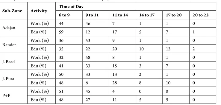
The percentage observation made in the survey for home base ongoing trip for the five sub-zones is as mentioned in the Table 8.
Table 8
Primary HBOT Generations on Temporal Basis (%)
Sub-Zone Activity Time of Day
6 to 9 9 to 11 11 to 14 14 to 17 17 to 20 20 to 22
Adajan Work (%) 44 46 7 1 1 0
Edu (%) 59 12 17 5 7 1
Rander Work (%) 36 53 9 1 1 0
Edu (%) 35 22 20 10 12 2
J. Baad Work (%) 32 58 8 1 1 0
Edu (%) 41 33 15 3 7 0
J. Pura Work (%) 50 33 13 2 1 0
Edu (%) 48 6 28 8 10 0
P+P Work (%) 51 45 4 0 0 0
Tapering of the trips for both work and education can be observed on the time axis. Higher percentages of work trips are generated in the first two time slots to cover almost 90% of the work trips against 70% of the education trips at the same time. The first time slots addresses the work trips pertaining to private service sectors where as second time slot from 9:00 AM to 11:00 AM covers trips of the institutes, government offices and trades activities. Surprisingly the shifts based worker component is not visible.
As most of the educational institutes in the Surat are in the morning session, high
percentages of trips are observed in the earlier morning slots. Pre-primary and primary institutes open 7:00 AM and Higher Secondary education institutes at 9:30 to 10:00 AM. Peaks are observed between 6 to 9 AM and 9 to 11 AM. They cover almost 70% of the trip generation. Third peak is around 12:00 PM where the colleges and universities are opening.
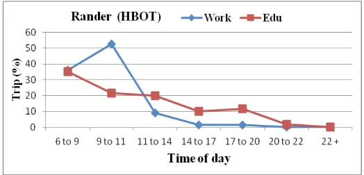
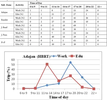
The typical work and education trips and there variations for two Sub-zones Adajan and Rander which are more populous are presented in the Fig. 4a and Fig. 4b.
Fig. 4a.
HBOT Generation Pattern of Adajan
Fig. 4b.
The influence of land use impact can be sensed in both the sub division of Adajan and Rander area respectively but trends remain same.
5.2.2. Home Base Return Trip (HBRT)
Pattern
The study observations in all the five sub-zones in the regard of Home Base Return
Journey are indicated in Table 9. It can be clearly seen a maximum returning work trips in the last two time slots of 17 to 20 hrs and 20 to 22 hrs where as maximum education trips are observed during 11 to 14 hrs and 14 to 17 hrs. It is nearly 50% of work trips between 17 to 20 hrs and 45-50% of education trips between 11 to 14 hrs. The trends of same are depicted in Fig. 5a and Fig. 5b for same two sub zones.
Table 9
Primary HBRT Generation on Temporal Basis
Sub- Zone Activity Time of Day6 to 9 9 to 11 11 to 14 14 to 17 17 to 20 20 to 22 22 +
Adajan Work (%) 1 1 8 11 55 24 0
Edu (%) 1 1 51 17 27 3 0
Rander Work (%) 0 0 0 18 45 36 1
Edu (%) 0 2 27 23 38 10 0
J. Baad Work (%) 0 0 11 10 69 7 3
Edu (%) 1 2 33 26 36 1 0
J. Pura Work (%) 0 0 7 13 54 24 2
Edu (%) 3 6 40 16 29 6 0
P+P Work (%) 0 0 4 5 65 25 0
Edu (%) 0 0 50 14 30 7 0
Fig. 5a.
Fig. 5b.
HBRT Generation Pattern of Rander
5.3. Development of Temporal Mandatory
Trip Generation Model
To know quantified trip generation with respect to time, there is need of modelling for various time slots for both categories of tour i.e. primary and secondary tour. In case of primary tours such as work, question of time choice is secondary as it is decided by external factors such type of job, working time prevailing with offices, firms and industries etc. in case of work. However there can be variation in case be activity duration in private sector or in personal business centres. Often there are shift timings in
certain industry to stagger out working time. Similarly time choice for the education trips depend on the opening and closing time of educational institutes and level of education. One can work out total working population from respective study area apportioning the work trips into six time slots from 6:00 AM to 10:00 PM, on the observed percentages.
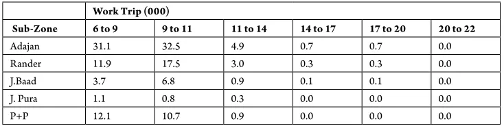
5.3.1. Trip Generations
The generated trips are magnitude in this regard for work and education purpose are shown in the Table 10a and Table 10b for all time slots.
Table 10a
HBOT Generation w. r. t. Time in a Day-Work
Work Trip (000)
Sub-Zone 6 to 9 9 to 11 11 to 14 14 to 17 17 to 20 20 to 22
Adajan 31.1 32.5 4.9 0.7 0.7 0.0
Rander 11.9 17.5 3.0 0.3 0.3 0.0
J.Baad 3.7 6.8 0.9 0.1 0.1 0.0
J. Pura 1.1 0.8 0.3 0.0 0.0 0.0
Table 10b
HBOT Generation w. r. t. Time in a Day-Education
Education Trip (000)
Sub-Zone 6 to 9 9 to 11 11 to 14 14 to 17 17 to 20 20 to 22
Adajan 34.36 6.99 9.32 2.91 4.08 0
Rander 11.12 6.99 6.35 3.18 3.81 0.64
J.Baad 4.64 3.74 1.7 0.34 0.79 0
J. Pura 1.08 0.13 0.63 0.18 0.22 0
P+P 10.78 6.07 2.47 1.12 2.02 0
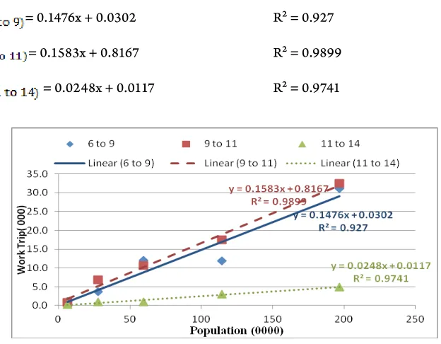
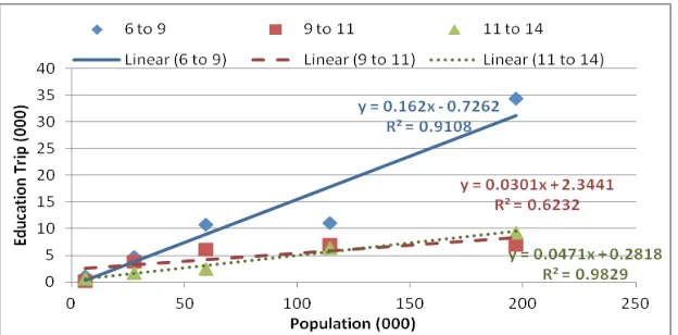
Regression models to relate the work for major time slots are now developed and presented in Fig. 6. On similar line Fig. 7 provide the relation between trip generation and population for education
purpose. The regression model and their statistical measure (R2) for both education
and work trips are mentioned below. y and x are work trips and population of sub zone.
For Work Trip
= 0.1476x + 0.0302 R² = 0.927
= 0.1583x + 0.8167 R² = 0.9899
= 0.0248x + 0.0117 R² = 0.9741
Fig. 6.
For Education Trip
= 0.162x - 0.7262 R² = 0.9108
= 0.0301x + 2.3441 R² = 0.6232
= 0.0471x + 0.2818 R² = 0.9829
Here, y = Education Trip, x = Population of Sub-Zone.
Fig. 7.
Temporal HBOT Generation MODEL-Education
5.3.2. Work and Education Trips Rates
The above data is further used to compute the per capita per day trip rates as mentioned below. The difference in rates in the time slots
Table 11
Work and Education Trip Rates in Morning Session
Sub-Zones Work-Trip Rate per Capita/Day Education Trip Rate/Capita/Day
6 to 9 9 to 11 11 to 14 6 to 9 9 to 11 11 to 14
Adajan 0.158 0.165 0.025 0.175 0.036 0.047
Rander 0.104 0.153 0.026 0.097 0.061 0.055
J.Baad 0.134 0.243 0.034 0.167 0.134 0.061
J. Pura 0.183 0.121 0.048 0.173 0.022 0.101
P+P 0.203 0.179 0.016 0.181 0.102 0.041
6. Conclusion
Conventiona l urban travel demand modelling adopted in most of cases to-date consider basic unit as trip rather tour, thereby missing time component. However it cannot be ignored in developing urban transportation plan in proper perspective. It should have activity based modelling framework to analyze activities pattern. Spatial and temporal activities aspect does matter in scheduling and strategic travel planning. So, trip generation should be related to activity based tours by household members. The present paper highlights the various aspects of activity based temporal trip generation modelling with reference to activity and travel pattern for various time segments. Focus in present work is on the mandatory or primary activities of work and education. The travel pattern of the primary tours have clearly indicated the higher share in the morning two slots for home based ongoing trips, where as higher proportion has been evening two slots for the return trips. Morning and noon slots have shown higher rates for the education trips. Spatial-Temporal work and education regression models are developed to relate the magnitude
for various time slots segment. Variation in trip rates for varied time slots are clearly visible to reflect on time factor. The model built here is to focus on activity based trip generations to provide the base for the next phases of activity based transport planning, which bears importance in near future.
References
Bhat, C.R.; Koppelman, F.S. 2003. Activity-Based Modeling of Travel Demand, Second Edition, Kluwer Academic publisher, New York.
Bhat, C.R.; Singh, S.K. 2000. A Comprehensive Daily Activity-Travel Generation Model System for Workers,
Transportation Research Part A: Policy and Practice. DOI: http://dx.doi.org/10.1016/S0965-8564(98)00037-8, 34(1): 1-22.
Bowman, J.L. 1998. The Day Activity Schedule Approach to Travel Demand Analysis, PhD Dissertation Report, Massachusetts Institute of Technology.
Davidson, W.; Donnelly, R.; Vovsha, P.; Freedman, J.; Ruegg, S.; Hicks, J.; Castiglione, J.; Picado, R. 2007. Synthesis of First Practices and Operational Research Approaches in Activity-Based Travel Demand Modelling, Transportation Research Part A: Policy and Practice. DOI: http://dx.doi.org/10.1016/j. tra.2006.09.003, 41(5): 464-488.
Jovicic, G. 2001. Activity based travel demand modelling-a literature study, Danmarks Transport Forskning.
McNally, M.G.; Rindt, C.R. 2007. The Activity-Based Approach, Institute of Transportation Studies, University of California, Irvine.
Pendyala, R. 2002. Time of day modelling procedure for implementation in FSUTMS, Final Report, Research Centre Florida Department of Transportation.
Ruey, M.W. 1997. An Activity-Based Trip Generation Model, PhD Unpublished Dissertation, University of Califronia Irvine.