warwick.ac.uk/lib-publications
Original citation:
Denrell, Jerker, Liu, Chengwei and Le Mens, Gaël. (2017) When more selection is worse.
Strategy Science, 2 (1). pp. 39-63.
Permanent WRAP URL:
http://wrap.warwick.ac.uk/85716
Copyright and reuse:
The Warwick Research Archive Portal (WRAP) makes this work by researchers of the
University of Warwick available open access under the following conditions. Copyright ©
and all moral rights to the version of the paper presented here belong to the individual
author(s) and/or other copyright owners. To the extent reasonable and practicable the
material made available in WRAP has been checked for eligibility before being made
available.
Copies of full items can be used for personal research or study, educational, or not-for-profit
purposes without prior permission or charge. Provided that the authors, title and full
bibliographic details are credited, a hyperlink and/or URL is given for the original metadata
page and the content is not changed in any way.
Publisher’s statement:
https://doi.org/10.1287/stsc.2017.0025
A note on versions:
The version presented here may differ from the published version or, version of record, if
you wish to cite this item you are advised to consult the publisher’s version. Please see the
‘permanent WRAP URL’ above for details on accessing the published version and note that
access may require a subscription.
Jerker Denrell
Warwick Business School, Scarman Road, University of Warwick, Coventry, CV4
7AL UK, [email protected]
Chengwei Liu
Warwick Business School, Scarman Road, University of Warwick, Coventry, CV4
7AL UK, [email protected]
Ga¨
el Le Mens
Department of Economics and Business, Universitat Pompeu Fabra, C/Ramn Trias
Fargas, 25-27, 08005 Barcelona, SPAIN, [email protected]
Abstract
We demonstrate a paradox of selection: the average level of skill among the survivors of selection may initially increase but eventually decrease. This result occurs in a simple model in which performance is not frequency dependent, there are no delayed effects, and skill is unrelated to risk-taking. The performance of an agent in any given period equals a skill component plus a noise term. We show that the average skill of survivors eventually decreases when the noise terms in consecutive periods are dependent and drawn from a distribution with a ‘long’ tail - a sub-class of heavy-tailed distribution. This result occurs because only agents with extremely high level of performance survive many periods and extreme performance is not diagnostic of high skill when the noise term is drawn from a long-tailed distribution.
Keywords: Organizational Evolution, Evolutionary Economics, Organizational Ecology
Acknowledgments:We are grateful for comments from Bill Barnett, Mike Hannan, Thorbjorn Knudsen, Dan Levinthal, Jim March, and Sidney Winter.
1. Introduction
Suppose you observe an industry with the purpose of identifying and imitating best practice. You know that firms do not change their capabilities much over time due to learning or forgetting. The population of firms changes over time as a result of entry and exit. Low performing firms tend to exit the industry whereas highly performing firms tend to stay in. When should you observe the industry? In the early stages of the industry? Later on, when many firms have exited? Or in the middle-stages? A standard evolutionary argument (‘survival of the fittest’) suggests that you should observe the firms remaining in the later stages of the industry as these firms have survived selection for a longer time and are likely to be the most capable. In this paper, we demonstrate that there are conditions under which learning from those who have survived for the longest possible time is suboptimal and that one would be better off learning from those who have survived for a shorter time.
Of course, it is well known that selection does not necessarily increase the proportion of the most capable firms – those that would have the highest performance in the long run, had they survived (Wright, 1931; Levins, 1968; Holland, 1975; Nelson & Winter, 1982, 2002). When the ‘fitness’ of a practice depends on how many others have adopted this practice or on the presence of specific organizational characteristics, an inferior practice could become dominant (Wright, 1931; Maynard Smith, 1982; Arthur, 1989; Carroll & Harrison, 1994; Levinthal, 1997). Similarly, when selection operates on short-term performance, it might eliminate practices with positive long-term effects, especially in changing environments or when firms can adapt (Levins, 1968; Elster, 1979; Nelson & Winter, 1982; Levinthal & March, 1981; Levinthal & Posen, 2007; Levinthal & Marino, 2015). Finally, selection can be biased against practices that lead to highly variable performance even if mean performance is high (Cohen, 1966; Denrell & March, 2001; Levinthal & Posen, 2007).
selection happens when luck has persistent effects. In contrast, when luck has non-lasting effects (e.g., the contribution of luck to performance changes from period to period), selection is efficient and leads to an increased prevalence of superior characteristics.
In this paper we focus on just one aspect of evolutionary explanations – selection – and leave out many other important aspects. In particular, the dynamics of skills and routines, which is central to the evolutionary theory of the firm (Nelson & Winter, 1982), is not explored here. Nelson & Winter (1982) assume that profitable firms expand while unprofitable firms contract. Moreover, they assume that unprofitable firms are more likely than profitable firms to search for new routines. Their focus is on how routines evolve as a result of such market driven search processes (Winter, 1971). Our focus is instead on the process of elimination of relatively poorly performing units. Using the terminology of Hodgson & Knudsen (2010), we focus on ‘subset’ selection (selecting a subset of units for survival, without changing their properties) while the evolutionary theory of the firm focuses on ‘successor’ selection (in which the units being selected change through imperfect replication involving mutation but also, in social science applications, processes of learning and search).
Evolutionary theories and selection explanations are sometimes viewed as alternative forms of ex-planations distinct from theories that emphasize goal-directed and adaptive behavior by managers. We do not pursue this agenda here. Our focus is on the population level consequences of selection regardless of the level of intentionality and rationality of the agents involved. Most selection models in economics and management assume that agents are intentional and goal-directed (Nelson and Winter, 1982, p. 10-11). And while many evolutionary accounts assume that agents are boundedly rational instead of profit maximizing (Alchian, 1950; Winter, 1964) there are several well-known selection models in economics that assume that agents are rational. For example, selection in the model of Jovanovic (1982) (i.e., exit by a firm) occurs as the result of optimal stopping based on Bayesian updating.
when our technical results are relevant and discuss the implications of our findings for empirical phenomena such as organizational obsolescence.
2. Illustration
To illustrate the basic idea, consider the following simple model. There aren= 50 firms. The performance of firm i in period t, pi,t, is equal to the sum of its skill, ui, and a noise term, εi: pi,t =ui+εi. There are two levels of skill: high (ui = 1), and low (ui = 0), each equally likely.
The level of skill and the value of the noise term remain constant during the lifetime of a firm. It follows that the performance of firmiis the same in every period. This setup represents a situation when initial ‘luck’ has strong long-term effects.
Selection works as follows. In each periodtthe 10 percent lowest performing firms (based onpi,t)
are removed from the population. Each eliminated firm is replaced by a new firm. Consider a new firmj. The probability that it has high skill (uj = 1) is 50% and its performance ispj,t=uj+εj
whereεj is drawn from the same densityfε. Note that bothuj andεj remain constant during the
lifetime of a firm. We are interested in how the proportion of high skill firms in the population evolves over time. Does it increase monotonically with time? Are older firms, that survived more selections, more likely to have high skill?
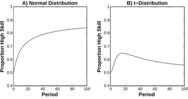
Figure 1A shows that when the noise terms are drawn from a normal distribution, the proportion of high skill firms increases over time. The pattern differs, however, when the noise terms are drawn from a Student’s t-distribution. As shown in Figure 1B, the proportion of high skill firms initially increases but eventually decreases and ultimately becomes close to 50%, the proportion of high skill firms at the beginning. What is noteworthy is that firms that have survived for a longer time (e.g., 100 periods) areless likely to have high skill (ui= 1) than firms that survived for a shorter
time (e.g., 20 periods). The mechanism underlying the dynamics depicted on Figure 1B thus leads to ‘inefficient’ selection. Although firms with the highest level of performance are more likely to survive in every period, and firms with high skill have higher expected performance, selection based on performance does not increase the proportion of high skill firms. In contrast, after some time, it leads to adecrease in the proportion of high skill firms.
0 20 40 60 80 100 0.4
0.5 0.6 0.7 0.8 0.9 1
Period
Proportion High Skill
A) Normal Distribution
0 20 40 60 80 100 0.4
0.5 0.6 0.7 0.8 0.9 1
Period
Proportion High Skill
[image:6.612.151.457.126.288.2]B) t−Distribution
Figure 1. Proportion of high skill firms as a function of time. In each period the
firms with the 10 percent lowest performances are removed and replaced with new firms. The noise terms remain the same across periods and are drawn from A) a normal distribution with mean 0 and variance 1 and B) a t-distribution with mean 0 and 1 degree of freedom. Each graph is based on 10,000 simulations, each with
n= 50 firms.
performance partly depends on luck and luck is drawn from a ‘long-tailed’ distribution, such as the t-distribution, an extremely high level performance is not diagnostic of high skill (Weibull et al., 2007; Denrell & Liu, 2012). Hence, having survived many periods can in fact be less diagnostic of high skill than surviving fewer periods. This is because surviving many periods requires an extreme level of performance, whereas surviving fewer periods requires a high but not extreme level of performance.
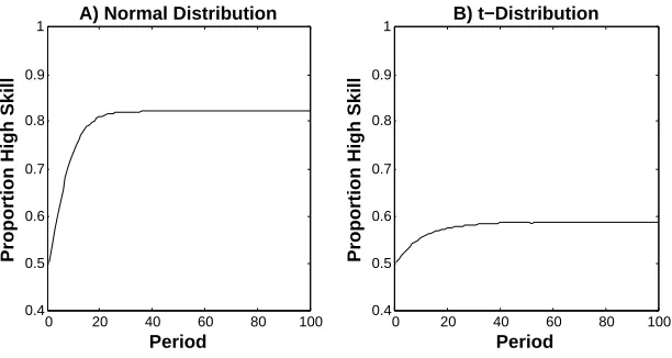
Importantly, this mechanism only operates when the performance in periodtis strongly depen-dent on the performance in prior periods (conditional on skill level). In particular, it does not apply when the noise terms are redrawn in every period. Consider the following variation of the model. As before, the performance of firm i in period t, pi,t, equals its skill, ui plus a noise term. But
here, we assume that the noise terms are not drawn just once at the time of entry but are redrawn in every period. Thus, we have a similar specification, but with a time index on the noise term
εi,t: pi,t =ui+εi,t. We assume that the noise terms areiid for allt andi. Figure 2 displays the
0 20 40 60 80 100 0.4
0.5 0.6 0.7 0.8 0.9 1
Period
Proportion High Skill
A) Normal Distribution
0 20 40 60 80 100 0.4
0.5 0.6 0.7 0.8 0.9 1
Period
Proportion High Skill
[image:7.612.151.457.125.288.2]B) t−Distribution
Figure 2. Proportion of high skill firms as a function of time. In each period the
firms with the 10 percent lowest performances are removed and replaced with new firms. The noise terms are redrawn in every period from A) a normal distribution and B) a t-distribution. Each graph is based on 10,000 simulations, each with
n= 50 firms.
proportion of high skill firms monotonically increases over time in both cases. In contrast to what happened in the previous setting (Figure 1B), selection is efficient even when the noise term follows a t-distribution (Figure 2B).
Why is the proportion of high skill firms monotonically increasing when noise terms are indepen-dently drawn in every period but not when they are drawn just once at the time of entry (in the case of a t-distribution)? When the noise terms are independently drawn in every period survival until the end of periodt requires that a firm passest distinct ‘tests’. All these tests are
indepen-dentconditional on skill. In this case, survival during early periods (the early ‘tests’) is informative
about skill since survival during these early periods does not require extreme levels of performances. By contrast, when the noise term is drawn just at the time of entry, allttests are dependent.
It is worth noting that inefficient selection can occur even when firm performance does not remain constant during the lifetime of a firm. For example, performance may follow a random walk (Levinthal, 1991; Denrell, 2004; Le Mens et al., 2011). Specifically, consider a firm that enters in periodt. Its performance in periodtfollows the same specification as before: εi,t: pi,t=ui+εi,t. Its
0 20 40 60 80 100 0.4
0.45 0.5 0.55 0.6 0.65 0.7 0.75 0.8
Period
Proportion High Skill
A) t−Distribution, w = 0.20
0 20 40 60 80 100 0.4
0.45 0.5 0.55 0.6 0.65 0.7 0.75 0.8
Period
Proportion High Skill
[image:8.612.148.459.124.288.2]B) t−Distribution, w = 0.35
Figure 3. How the proportion of high skill firms changes over time when the
noise term follows a random walk and A)εi,t are drawn from a t-distribution with
1 degree of freedom andw= 0.2 and B)εi,tare drawn from a t-distribution with 1
degree of freedom and w= 0.35. Each graph is based on 10,000 simulations, each with 50 firms, where thewpercent firms with the lowest performances are replaced in every period.
is not constant but changes in every period. Simulations show that if selection is strong enough (w, the proportion of firms that exit in each period, is high enough), the proportion of high skill firms will decline with time after some time (see Figure 3 for a depiction of the dynamics of this proportion for two levels ofw). More generally, in Sections 6 and 7 we show that our basic result holds under a number of alternative assumptions about selection, replacement, and performance dynamics.
3. Prior Literature on The Efficiency of Selection
become buffered from selection forces (Levinthal, 1991; Barnett, 1997). Other researchers have demonstrated that even if selection processes reliably select on the basis of economic performance, the most efficient organizations may fail to survive. As Levinthal and Posen write: ‘Even if selection is effective in removing inferior organizations at one point in time, it may be ineffective over time in that it may remove organizations that, had they survived, would have gone on to do well.’ (Levinthal and Posen, 2007, p. 587). Two well-known mechanisms leading to such inefficient selection are time-dependent fitness and frequency-dependent fitness.
Consider time-dependent fitness. Fitness may change over time because firms or their environ-ments change, but selection is often myopic and responds only to current levels of fitness (Elster, 1979; Levinthal & March, 1981; Levinthal & Posen, 2007). Such myopic selection may eliminate units with high future potential but low current performance. As Nelson and Winter note: ‘[i]f firms are small in the early stages of industry growth, those that start with techniques that are efficient only after the firm has grown considerably may be defeated in the evolutionary struggle by firms whose techniques are better suited to low levels of output’ (Nelson & Winter, 1982: 159). Building upon this insight, Denrell and March (2001) showed that practices that improve by learning-by-doing may be selected against because of their poor initial performance. In their simulation firms were endowed with one of two possible technologies. The first technology generated a fixed payoff. The second technology generated a low initial payoff but its payoff increases over time. Even if the long-term payoff of the second technology is higher than the fixed payoff of the first technology, im-plying that the second technology is ‘superior’, firms with the second technology were likely to fail before the potential of their technology was revealed. As a result, the proportion of firms with the second technology decreased over time. Selection is inefficient in this case because the proportion of firms with the second technology, which has a higher long-term payoff, is reduced over time. The inefficiency occurs because the fitness of the second technology changes systematically over time and the selection process is myopic in the sense that it reacts only to current payoffs and not to anticipated future payoffs.
1997). Carroll & Harrison (1994) showed, in an evolutionary model, how frequency dependence allows inefficient organizational forms to survive. Following past empirical work, they assume that both the founding and mortality rates are frequency (density) dependent. Organizational forms only differ in their competitive effects: the negative effect thatone organization of form i
exerts on organizations of formj. An organizational formi is superior to an organizational form
j if the competitive effect of i is larger than the competitive effect of j. Their simulations show that whenever an inferior form emerges earlier than a superior form it can become dominant. The intuition is that the inferior form exerts a largertotalcompetitive pressure on the superior form, than vice versa, because there are more organizations of the inferior form (higher density). Simulations of their model show that when the inferior form enters first the density of the superior form initially increases but eventually declines to 0. The density of the superior form initially increases because, at this stage, the density of the inferior form is not yet very high. The decline occurs because when the inferior form becomes numerous it exerts a high total competitive pressure on the superior form. This scenario also represents a kind of ‘inefficient’ selection. The superior form is eliminated because there are more organizations of the inferior form and performance depends on the number (frequency) of organizations of the same form.
Variability is another reason why selection may not increase the proportion of a trait with the highest expected performance. It is well-known in evolutionary theory that a trait associated with the highest level of expected performance may be selected against if its performance is also highly variable (Cohen, 1966; Yoshimura & Clark, 1993; Cvijovic et al., 2015). Similarly, management theorists have argued that an organizational practice with the highest expected performance may be decrease over time as a result of selection if this form also has the highest variance in performance. In particular, Levinthal & Posen (2007) and Levinthal & Marino (2015) have shown that adaptive learning processes may be selected against because they imply increased variability in performance as a result of the adjustments the firm will go through. Adaptive learning may lead to superior average performance in the long run but may lead to a higher variability in performance in the short run. Higher variability, in turn, increases the chances of elimination in the short-run, before the long-term advantages have been realized.
We show that even in this case there exist conditions under which selection will be inefficient in the sense that the proportion of agents with the superior trait does not necessarily increase over time. To the contrary, the proportion of agents with the superior trait ultimatelydeclines over time.
It is important to note that our model does not imply that less ‘fit’ firms are more likely to survive. In each period selection removes firms with low performance levels, consistent with the idea of the ‘survival of the fittest’ if fitness is measured in terms of performance. Indeed, because poorly performing firms are replaced, average performance in the population increases over time, implying that the population becomes more ‘fit’ over time. The fact that the population becomes more ‘fit’ over time, however, is equally true for other mechanisms of inefficient selection, such as time-dependent fitness. Selection may reduce the proportion of the technology with highest long-term performance but average performance can nevertheless increase over time if the performance of the inferior technology also improves over time.
If selection leads to a monotonic performance increase over time in our model, why does it matter that the proportion of firms with high skill (ui= 1) decreases over time? For an observer
interested only in average performance, the systematic decline inuiover time may not matter. The
decline inui over time would matter for an observer interested in identifying practices and skills
that contribute to high performance. If ui represents the capability of a firm, whileεi represents
situational influences beyond the control of management, such an observer would be interested in learning from firms with high capabilities (ui = 1). Our results imply that such an observer should
not imitate firms that have been through many rounds of selection. In Section 8 we discuss in more detail when our results do and do not matter.
4. Formal Analysis I: Selection and No Replacement
To analyze when and why selection can reduce the proportion of the type with the highest value of ui we first focus on a simple setting when there is selection but no replacement. That is, we
analyze the effect of repeated selection on a cohort of agents. In Section 6.1 we show that the basic result continues to hold if there is also replacement.
4.1. Model. Consider a population of infinitely many agents (an agent can be an individual, a firm etc.). Assuming that a population is made of infinitely many agents is a standard assumption in many evolutionary models that allows for mathematical tractability. Our illustrative graphs in Section 2 showed that we get similar results in a population of 50 agents.
Agents are either high skill agents (ui = 1) or low skill agents (ui = 0). The level of skill
0.50. We use the label ‘skill’ to denote a trait that contributes to the performance of agenti. The performance of agent iin period t, pi,t, equals her skill,ui plus a noise term, εi: pi,t =ui+εi,t.
The noise term represents an aspect of performance beyond the control of the agent. We assume that the noise term is drawn from a densityfεwith positive variance. We assume that the support
offε is of the form (a,+∞) with a∈ {−∞,R}.1 Note that while we use the label ‘noise term’ for
εi, we do not assume that the expected value offεhas to be equal to 0.
Selection works as follows. In each periodt, thew percent agents with the lowest performance levels (lowest values ofpi,t) are removed from the population.
We denote byπtthe proportion of high skill agents at the end of periodt. We denote byπ0 the
initial proportion of high skill agent (π0= 0.50). We are interested in how πt evolves witht. Does
it increase witht implying that selection increases the proportion of agents with high skill?
4.2. Independent Noise Terms. Suppose the noise terms are independent across agents and periods. That is, pi,t =ui+εi,t, andεi,t are iid draws from the density fε for all t and i. We
denote the density of the performance distribution of high skill agents byf1and the density of the performance distribution of low skill agents by f0. Because the noise terms are redrawn in every
period, the distribution of performance conditional on skill remains constant. Hence, we have:
f0(pi,t+1) =f0(pi,t),
and
f1(pi,t+1) =f1(pi,t).
It follows that, in every period, high skill agents (whose performances equalpi,t = 1 +εi,t) are
likely to have a higher performance than low skill agents (whose performances equalpi,t=εi,t). As
a result, the proportion of high skill agents increases over time. Theorem 1 demonstrates that this holds for any (continuous) distribution of the noise term:
Theorem 1. Supposepi,t=ui+εi,t, where, for allt andi,εi,t are iid draws from the continuous
densityfε. Wheneverw∈(0,1) expected skill increases over time: πt+1> πt for allt≥1.
Proof. See Appendix A.
4.3. Constant Noise Terms. Suppose now that the noise terms remain the same in all periods. The noise term in the first periodεi,1is drawn from densityfε. The noise terms in periods 2,3,4, ...
1Ancillary analyses and computer simulations show that most of our results still apply when the support off
εhas an
are identical to the noise term drawn in period 1. The performance of agentithus remains the same in all periods: For allt, pi,t =ui+εi,1. This setup represents a situation of extreme dependency
across periods. Such dependency can occur when initial ‘luck’ has long-term effects.
An important implication of this specification is that the distribution of performance conditional on skill and survival systematically changes over time. The reason is that selection in prior periods eliminates agents with low values of pi,t and thus indirectly eliminates agents with low values of εi,1. Whether selection increases average skill or not then depends on the nature of the distribution
of the noise term (fε).
The following theorem shows that whether selection leads to a monotonic increase in the pro-portion of high skill agents or not depends on whether the hazard function of the noise distribution is an increasing function or not. The hazard functionhof a distributionf is defined as the ratio of the density over 1 minus the cumulative density functionF: h(x) =f(x)/(1−F(x)).
Theorem 2. Supposepi,t =ui+εi,1 andεi,1 is drawn from density fε. Let hε denote the hazard
function of distributionfε. In this case,
i) The proportion of high skill agents increases as a result of selection during the first period:
π1> π0= 0.5
ii) The evolution of the proportion of high skill agents after the first period (t >1) depends on the
shape of the hazard function of the noise distribution:
a) Ifhε is an increasing function, thenπtincreases with t.
b) Ifhε is a decreasing function, thenπt decreases with t fort large enough,
c) If there existsc∗ such that h
ε(c−1)< hε(c)for allc < c∗ andhε(c−1)> hε(c)for all c > c∗,
πt decreases with tfort large enough.
d) If there exists c∗ such that hε(c−1) = hε(c) for all c > c∗, πt remains constant for t large
enough.
Proof. See Appendix B.
Log-normal distribution, the Inverse Gaussian, the Weibull distribution with parameterk <1, and the Pareto distribution. There exists distributions, such as the Laplace distribution, which has fatter tails than the normal distribution but which nevertheless does not have a decreasing hazard function.
Table 1. Shape of the hazard functions of a set of distributions.
Distribution Shape of the Hazard Function Uniform Increasing
Normal Increasing Logistic Increasing Poisson Increasing Extreme Value Increasing Exponential Constant
Laplace Initially increasing, eventually constant Cauchy Initially increasing, eventually decreasing Log-normal Initially increasing, eventually decreasing Inverse Gaussian Initially increasing, eventually decreasing
Weibull Increasing whenk >1, decreasing whenk <1 Pareto Decreasing
4.4. Long-Tailed Distributions. Theorem 2 shows that the proportion of high skill agents will eventually decline over time when the noise term is drawn at time of entry from a distribution with a hazard function which is (eventually) decreasing. This raises the question of which distributions have a declining hazard function. Can these be characterized in some intuitive way? In this section we show that a class of distributions, called ‘long-tailed’ distributions, have exactly the properties we seek.
Formally, a random variableX has a long-tailed distribution if (1−Fx(c+y))/(1−Fx(c))→1
asc→ ∞for ally >0 (Foss et al., 2013). HereFx() denotes the cumulative distribution function
ofX. The property of having a long tail thus corresponds to the fact that ifX is larger than some very large constantc (which occurs with probability 1−Fx(c)) then X is also likely to be larger
than c+y (which occurs with probability 1−Fx(c+y)). Examples of long-tailed distributions
include the t-distribution with one degree of freedom (i.e, the Cauchy distribution) but also the Pareto distribution and the Log-normal distribution.
level of performance among the agents that were eliminated in periodt. All survivors during period
t have a performance above p∗t. When the noise terms remain constant the proportion of high skill agents among the survivors of t periods is P(ui = 1 | pi > p∗t), the proportion of high skill
agents among agents that have a performance abovep∗
t. The property of being long-tailed precisely
captures the set of noise term distributions for whichP(ui = 1|pi > p∗t) becomes uninformative
about skill asp∗t becomes large. Formally,
Theorem 3. Letpi=ui+εi whereui= 1with probability 0.5 and ui= 0otherwise. Then,
i)limc→∞P(ui= 1|pi> c) = 0.5 if and only iffεis the density of a long-tailed distribution.
ii)limt→∞P(ui= 1|pi> p∗t) = 0.5 if and only iffε is the density of a long-tailed distribution.
Proof. See Appendix C.
Theorem 3 implies that the proportion of high skill agents will converge to 50%, the initial proportion, when the noise term is drawn from a ‘long-tailed’ distribution.
What about the condition regarding the hazard function? Theorem 2 states that average skill eventually declines if the hazard function of the noise term distribution is eventually declining. It turns out that the property of having a long tail also implies that the hazard function is (eventually) declining. Formally, if a distribution is long-tailed then its hazard functionh(x) will eventually go to 0: h(x)→0 asx→ ∞(Nair et al., 2013).
How does the property of being long-tailed relate to the more widely known concept of ‘fat-tailed’ distributions? A distribution is ‘fat-‘fat-tailed’ if the upper tails behaves as a power law, i.e.,
if P(x > c) ≈ c−x as c → ∞ (Foss et al., 2013). Fat-tailed distributions belong to the class
of ‘heavy’ tailed distributions (all fat-tailed distributions are tailed but there exists heavy-tailed distributions which are not fat-heavy-tailed). Informally, a distribution is heavy-heavy-tailed if its tail is heavier than the tail of an exponential distribution.2 Long-tailed distributions are a sub-class of ‘heavy-tailed’ distributions (Nair et al., 2013). Hence, all long-tailed distributions are heavy tailed. There exist long-tailed distributions, however, which are heavy-tailed but not fat-tailed (an example is the Log-normal distribution).
5. Intuition
Why does selection increase the proportion of high skill agents if the noise terms are redrawn but can decrease the proportion of high skill agents if the noise terms are constant? And why does
the effect of selection depend on the hazard function of the noise term? The basic result can be explained in two different ways.
5.1. Intuition 1: The Diagnosticity of Survival Decreases with Time. The first type of explanation focuses on the skill levels of the survivors. After several periods of selection only a small fraction of the initial population remains. These survivors have had high performance during several periods. Is such high performance a reliable indication of high skill? This is not generally the case. It is well-known in statistics that a higher outcome may not indicate a higher expected value (Karlin & Rubin, 1956). For some ‘heavy-tailed’ noise term distributions a very high outcome may indicate a lower expected value than a moderately high outcome does (Weibull et al., 2007; Denrell & Liu, 2012). The reason is that extreme outcomes depend relatively more than moderately high outcomes on luck than skill. Survival during many period can, for similar reasons, be an unreliable indicator of high skill.
To explain this, consider the agents that have survived during all of the first t periods. What is the proportion of high skill agents among these survivors? Consider first the case when noise terms are constant. Performance in consecutive periods does not change (because the noise term remain constant). Moreover, because selection removes the agents with the lowest performances, the threshold for survival,p∗t, defined as the maximum level of performance among the agents that
failed in periodt, increases over time (See Lemma 4 in the Appendix). This implies that if an agent had a performance above the threshold in periodt(pi,t > p∗t), her performance was also above the
threshold in any previous period (pi,t−1> p∗t−1). The probability of survivingtperiods for an agent
with skillui =k is thus simply the probability that the performance drawn in the first period is
above the threshold in period t: P(pi,t > p∗t | ui =k). When the noise terms are constant, the
proportion of high skill agents among the survivors is thus
πt=P(ui = 1|pi,t> p∗t) =
P(pi,t> p∗t |ui= 1)P(ui= 1)
P(pi,t> p∗t |ui= 1)P(ui= 1) +P(pi,t> p∗t |ui= 0)P(ui= 0)
When the noise terms are constant the only thing we know about the agents that have survived fortperiods is that the performance they drew at the start was abovep∗t, the threshold for survival in periodt. When t is large, the value ofp∗t will be high. Hence, we know that the performance levels of all the survivors are very high. But the fact that they all have a high level of performance does not imply that they are all high skill agents. It is not generally true that the proportion high skill agents is higher among agents with higher levels of performance.
0 5 10 15 20 25 30 −1 0 1 2 3 Period Threshold (c)
A: Normal Distribution
0 5 10 15 20 25 30
−4 −2 0 2 4 6 8 Period Threshold (c) B: t−Distribution
−5 0 5 10
0.5 0.6 0.7 0.8 0.9 1 Threshold (c)
P[u =1 | p > c]
−5 0 5 10
0.5 0.55 0.6 0.65 0.7 Threshold (c)
P[u =1 | p > c]
Figure 4. Upper panels: Survival threshold as a function of time. Lower
quad-rants: Proportion of high skill agents among those with a performance above the threshold. Left panels: Noise term is drawn from a Normal distribution with mean 0 and variance 1. Right quadrants: Noise terms are drawn from a t-distribution with mean 0 and 1 degree of freedom.
a t-distribution. The lower quadrant shows how the proportion of high skill agents that have a performance above a threshold P(ui = 1 |pi,t > c) varies with the threshold, c. When the noise
term is drawn from a normal distribution P(ui = 1| pi,t > c) increases with c. When the noise
term is drawn from a t-distribution P(ui = 1 |pi,t > c) eventually declines with c and converges
to 0.5 asc→ ∞. As Theorem 3 shows, limc→∞P(ui = 1|pi,t > c) = 0.5 if and only iffε is the
density of a long-tailed distribution.
The situation differs when the noise terms are independently drawn in each period. In this case, survival during many periods does not become uninformative. To explain why, note that in this case performance changes every period because the noise terms are redrawn in every period. Moreover, conditional upon skill, performance levels in different periods are independent. The probability of survival duringtperiods for an agent with skill ui=k is thus the probability of surviving period
1,P(pi,1 > p∗1 |ui=k), multiplied by the probability of surviving period 2,P(pi,2> p∗2|ui=k),
etc. The proportion of high skill agents among the survivors oftperiods can thus be written as
πt=
P(pi,1> p∗1, ..., pi,t> p∗t |ui= 1)P(ui= 1)
P(pi,1> p∗1, ..., pi,t> p∗t |ui= 1)P(ui = 1) +P(pi,1> p∗1, ..., pi,t> p∗t |ui= 0)P(ui= 0)
Noting thatP(ui = 1) = P(ui = 0) = 0.5 and that performance levels in successive periods are
independent from each other conditional on skill, we can write:
πt=
Qt
j=1P(pi,j> p∗j |ui= 1)
Qt
j=1P(pi,j> p∗j |ui = 1) +Q
t
j=1P(pi,j> p∗j |ui= 0)
.
In contrast to the case of constant noise terms, this expression does not only depend on the proba-bility that the final performance is above the final threshold,P(pi,t> p∗t |ui=k), but also on what
happened in all prior periods. Moreover, because the performance in periodtis independent from performance in earlier periods, conditional on skill, more information is available compared to the case when the noise terms are constant. Stated differently, when the noise terms are independent an agent has to pass t independent tests to survive during t periods. While the test in the final period may be relatively uninformative about skill, becausep∗t is very high in that period, the early tests, whenp∗t is moderately high, remain informative.
5.2. Intuition 2: Failure Rates Conditional on Skill Change over Time. While the first explanation that focused on the diagnosticity of survival provides an intuition for why the proportion of high skill agents may eventually decrease when noise terms are constant and drawn from a long-tailed distribution, it does not explain why the hazard function of the noise term matters. We now provide an intuition for this.
In every period,wpercent of all agents ‘fail’ and are removed from the population. The change in the proportion of high skill agents depends on the proportion of high skill and low skill agents among the failures. Suppose, for example, that almost all of the agents that fail have low skill. In this case, it is intuitively clear that the proportion high skill agents among the survivors will increase. More generally, if the probability of failure is higher for low skill agents, the proportion of low skill agents decreases and hence average skill increases (see Lemma 1 in Appendix A).
To understand when selection increases the proportion of low skill agents, we thus need to understand when low skill agents are, in every period, less likely to fail than high skill agents. An agent fails whenever its performance is among thewpercent lowest performances. Ifp∗t+1 is defined as the maximum performance among the failures in periodt+ 1, we can say that an agent fails in periodt+ 1 whenever its performance in periodt+ 1 is at or belowp∗t+1.
The difference between high and low skill agent can then be stated as follows. 1) A low skill agentj (with skill equal touj= 0) fails in periodt+ 1 wheneverεj,t+1≤p∗t+1. The probability of
failure in period t+ 1 for a low skill agent is thus the probability thatεj,t+1 is at or belowp∗t+1.
Formulated differently: a high skill agentifails whenεi,t+1 is at or belowp∗t+1−1. The probability
of failure in period t+ 1 for a high skill agent is thus the probability that εi,t+1 is at or below p∗t+1−1. This formulation holds the key to understanding the difference between independent and constant noise terms.
Consider the case with independent noise terms. The noise terms are, for all agents and all periods, drawn from the same distribution. So the noise term for a high skill agent i, εi,t+1, is
drawn, in all periodst+ 1, from a distribution identical to that of εj,t+1, the noise term for a low
skill agent j. Because εi,t+1 and εj,t+1 are independently drawn from the same distribution it is
clear that the probability the low skill agent fails is higher than the probability that the high skill agent fails: P(εj,t+1 ≤p∗t+1)> P(εi,t+1 ≤p∗t+1−1). Because this holds for any periodt+ 1, the
proportion of high skill agents always increases (as long as the proportion of high skill agents is below 1).
Consider now the case with constant noise terms. Let us first focus on the probability that a low skill agent fails in period 2. A low skill agent j fails in period 2 (and not in period 1) if its performance is sufficiently high in period 1 and its performance in period 2 is at or below the threshold for survival. Formally, a low skill agent j fails in period 2 if pj,1 = εj,1 > p∗1 and pj,2 =εj,1 ≤p∗2. What matters for failure in period 2 is thus the distribution of performance in
period 2conditional on survival during period 1.
Suppose now that p∗2 = p∗1+y, where y > 0. Agents with a performance above p∗1 and at or belowp∗1+y, for somey >0, fail in period 2. The probability that a low skill agentj, who survived period 1, fails in period 2 falling is thus
P(p∗1+y≥pj,1> p∗1|pj,1> p∗1, uj = 0) =
P(p∗1+y≥pj,1> p∗1|uj= 0)
P(pj,1> p∗1, uj = 0)
.
Becausepj,1=εj,1 whenuj = 0 this conditional probability equals
(1) P(p∗1+y≥pj,1> p∗1|pj,1> p∗1, uj = 0) =
P(p∗1+y≥εj,1> p∗1)
P(εj,1> p∗1)
.
Imagine now that w is small. Only a small fraction of all agents are eliminated in each period. Thus only agents with a performance just above top∗1 (the threshold in period 1) are eliminated during period 2. That is, y is close to 0. Formally, let y →0 in equation 1. Asy →0, the right hand side converges tohε(p∗1) =fε(p∗1)/P(εj,1> p∗1), the hazard function of the noise distribution
atp∗
1 (Ross (2000), p. 220).
Now, let us focus on the probability that a high skill agent fails in period 2. A high skill agent
agent fails in period 2 thus depends on the distribution of performance conditional upon survival during period 1: fpi,1|pi,1>p∗1(pi,1 |pi,1 > p
∗
1). Again, suppose that p∗2 =p∗1+y. The probability
that a high skill agenti, who survived period 1, fails in period 2 is
P(p∗1+y≥pi,1> p∗1|pi,1> p∗1, ui = 1) =
P(p∗1+y ≥pi,1> p∗1|ui= 1)
P(pi,1> p∗1, ui = 1)
.
Becausepi,1= 1 +εi,1, this conditional probability equals
P(p∗1+y≥pi,1> p∗1|pi,1> p∗1, ui= 1) =
P(p∗1+y−1≥εi,1> p∗1−1)
P(εi,1> p∗1−1)
.
Asy→0 this expression converges tohε(p∗1−1) =fε(p∗1−1)/P(εi,1> p∗1−1), the hazard function
of the noise distribution atp∗1−1.
In summary, whether low skill or high skill agents are more likely to fail during period 2 depends on the hazard function of the noise term distribution. Low skill agents are more likely to fail than high skill agents are if the hazard function atp∗
1,hε(p∗1), is larger than the hazard function atp∗1−1, hε(p∗1−1). It follows that low skill agents are more likely to fail than high skill agents whenever
hε(x) > hε(x−1), i.e., whenever the hazard function of the noise distribution is an increasing
function.
This result can be restated in terms of the hazard functions for the performance distributions of low and high skill agents. The hazard function of the performance distribution for a low skill agent,
hpj,t,u=0(x), is equal to the hazard function for the noise distribution,hε(x) sincepj,t=εj,1for low skill agents. The hazard function of the performance distribution for a high skill agent,hpi,t,u=1(x), is equal to the hazard function for the noise distribution evaluated atx−1,hε(x−1), since the
equationεj,1=pi,t−1 holds for high skill agents. It follows that the inequalityhε(x)> hε(x−1)
for allxcan be restated ashpj,t,u=0(z)> hpi,t,u=1(z) for allz, i.e., the hazard function for low skill agents always lies above the hazard rate function for high skill agents.
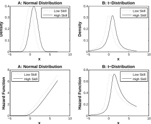
As Figure 5A shows, the hazard function is an increasing function when the noise term is drawn from a normal distribution. Moreover, the hazard rate function for low skill agents always lies above the hazard rate function for high skill agents. As a result, a low skill agent is, in every period, more likely to fail than a high skill agent. To demonstrate this, Figure 6 plots how the probability of failure varies over time for high and low skill agents (for the case when there is only selection and no replacement). Specifically, Figure 6 plots the probability of failure conditional on survival,
P(pi,t ≤ p∗t | ∀j < t : pi,j > p∗j, ui = k) for high and low skill agents. The probability of failure
−5 0 5 10 0 0.1 0.2 0.3 0.4 x Density
A: Normal Distribution
Low Skill High Skill
−5 0 5 10
0 0.1 0.2 0.3 0.4 x Density B: t−Distribution Low Skill High Skill
−5 0 5 10
0 2 4 6 8 x Hazard Function
A: Normal Distribution
Low Skill High Skill
−5 0 5 10
[image:21.612.151.458.96.348.2]0 0.2 0.4 0.6 0.8 x Hazard Function B: t−Distribution Low Skill High Skill
Figure 5. Upper panels: Density of performance for low and high skill agents when the noise distribution is drawn from A) a normal distribution and B) a t-distribution. Lower panels: hazard functions for high and low skill agents.
the high skill agents eventually becomes higher than the hazard function for the low skill agents (Figure 5B). The implication of such crossing hazard function is that the probability of failure will eventually become higher for high skill agents than for low skill agents (Figure 6B).
0 5 10 15 20 25 30 0
0.02 0.04 0.06 0.08 0.1 0.12 0.14 0.16 0.18 0.2
Period
Failure Probability
A: Normal Distribution
0 5 10 15 20 25 30 0
0.02 0.04 0.06 0.08 0.1 0.12 0.14 0.16 0.18 0.2
Period
Failure Probability
B: t−Distribution
High Skill Low Skill
[image:22.612.143.462.101.264.2]High Skill Low Skill
Figure 6. How the failure probability (when there is no replacement) varies over
time for high and low skill agents when the noise terms are constant and drawn from A) a normal distribution and B) a t-distribution. Minor oscillations in the graphs are due to numerical imprecision in the computations.
surviving high and low skill agents have almost identical performance distributions and hence are equally likely to fail.
survival during many periods, even if it would require extreme high levels of performance, is still diagnostic of high skill.
6. Alternative Assumptions about Selection and Replacement
The model on which our formal analysis has focused is admittedly a toy model that hardly maps onto any naturally occurring settings. Do our results also hold in more realistic settings? Here we explore this issue by simulating models with different assumptions about how selection and replacement operates.
6.1. Replacement. Our main result about the emergence of a non-monotonic pattern in the pro-portion of high-skill agents also holds when the agents who exit the population are replaced by new agents. More specifically, consider the setting of Section 4.3 where the noise terms are constant. Here, we assume that everything remains the same, except that each eliminated agentiis replaced by a new agent j with performance pj = ui+εj where εj is independently drawn from density fε(ε). The probability that a new agent has high skill (uj = 1) is 50%. We have:
Theorem 4. Theorem 2 holds in this setting as well.
Proof. See Appendix D.
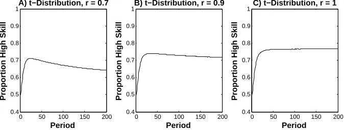
6.2. Replacement from a changing skill pool. We have assumed that the probability that a new agent has high skill is 50% in all periods. Entrants may learn from survivors, however. If so, the probability that an entrant has high skill may increase over time. To model this, suppose the probability that a new agent entering in periodt has high skill equals qt =rπt+ (1−r)0.5.
The probability that a new agent entering in period t has high skill is thus a weighted average between the proportion of agents with high skill among the survivors (πt) and 50%. The weight on πt isr∈[0,1]. It can be interpreted as the probability that an entrant is able to copy a survivor.
0 50 100 150 200 0.4
0.5 0.6 0.7 0.8 0.9 1
Period
Proportion High Skill
A) t−Distribution, r = 0.7
0 50 100 150 200 0.4
0.5 0.6 0.7 0.8 0.9 1
Period
Proportion High Skill
B) t−Distribution, r = 0.9
0 50 100 150 200 0.4
0.5 0.6 0.7 0.8 0.9 1
Period
Proportion High Skill
[image:24.612.138.475.151.279.2]C) t−Distribution, r = 1
Figure 7. How the proportion of high skill agents changes over time in a simu-lation when there is replacement from a changing skill pool, the noise terms are drawn from a t-distribution with 1 degree of freedom,w= 0.1, and A)r= 0.7, B)
r= 0.9 and C)r= 1 (based on 10,000 simulations, each with 50 agents).
6.3. Probabilistic selection. The models examined so far assumed that all agents with the lowest
wpercent performances were eliminated and replaced in each period. It may be more realistic to assume that selection operates in a probabilistic fashion: agents with relatively low performance are more likely than agents with relatively good performance to fail and be replaced. To model this, let
pwt be the level of performance such thatwpercent of all agents have a lower level of performance in
periodt. Previously we assumed that all agents with a performance at or belowpwt were eliminated
and all agents with a performance abovepwt survived. To model probabilistic selection we assume instead that the probability that agentisurvives period tis 1/(1 +exp(−s(pi,t−pwt)). Heres≥0
is a parameter that regulates the extent to which selection is sensitive to relative performance. A larger value of simplies that the probability of survival is more sensitive to relative performance (pi,t−pwt). Whens → ∞ all agents with a performance abovepwt survive and all agents with a
performance below that threshold are replaced. Whens= 0, the probability of survival equals 0.5 for all agents and is thus unrelated to relative performance.
Simulations show that the basic result hold even for probabilistic selection unless the value of
s is low. To illustrate this, suppose w = 0.1. Here, pwt is equal to the tenth percentile of the
0 0.5 1 0 0.2 0.4 0.6 0.8 1 Percentile Survival Probability
A) Effect of s
0 50 100
0.4 0.45 0.5 0.55 0.6 0.65 0.7 0.75 0.8 Period
Proportion High Skill
B) t−Distribution, s = 1
0 50 100
0.4 0.45 0.5 0.55 0.6 0.65 0.7 0.75 0.8 Period
Proportion High Skill
C) t−Distribution, s = 0.1
[image:25.612.131.484.137.275.2]s = 1 s=0.1
Figure 8. A) The impact of the value ofson the probability of survival. B) and C) How the proportion of high skill agents changes over time when the noise term is drawn from a t-distribution with B) s = 1 and C) s = 0.1 (based on 10,000 simulations, each with 50 agents).
0.5 for a performance level equal to the tenth percentile (i.e., pi,1 =p01.1). If s = 1 the survival
probability quickly increases towards one for higher performance levels while ifs= 0.1 the survival probability remains at a moderate level (around 55%) unless performance is very high. Panels B and C in Figure 8 show how the proportion of high skill agents changes over time whens= 1 and
s= 0.1. In each simulation there aren= 50 agents, high and low skill are initially equally likely, the noise terms are constant during the life-time of an agent, and each eliminated agent is replaced with a new agent. The proportion of high skill agents initially increases but eventually declines whens = 1. Whens= 0.1, and even high performing agents may fail to survive, the proportion initially increases but then reaches a plateau.
The implication is that the proportion of high skill agents can only decrease if survival depends on relative rather than absolute performance.
6.5. Size Changes. Our model focused on the elimination of poorly performing units and assumed that all agents were of equal size. In contrast, several evolutionary models in management have focused on growth. For example, Nelson and Winter (1982) explored the consequences of the assumption that profitable firms grow and unprofitable firms contract. Changes in traits among survivors may be relatively uninteresting in such a model. What matters are size-weighted traits: whether large firms are more likely to use ‘efficient’ technologies.
Do our results hold also in a model where relative performance determines growth? To explore this, we simulated a simple version of a model in which relatively high performance leads to growth in size while relatively low performance leads to contraction in size. The model is specified as follows. There aren= 50 firms. The performance of firmiispi=ui+εi. There are only two levels
ofui: high (ui= 1) and low (ui= 0), each equally likely. The level ofui remains the same during
the life-time of a firm. So does the noise term,εi. There is no selection in this model: we ignore
selection to focus on size changes. All firms survive all periods and there are no entrants. Firms do change in size, however. At the start, each firm has size si,1 = 1. Firm size changes, in each
period, as follows. Letztbe the market share weighted performance in period t: zt=P n
i=1mi,tpi
where mi,t = si,t/P n
i=1si,t is the market share of firm i at the start of period t. Every firm
with performance above zt increases in size by 10%: if pi > zt then si,t+1 = 1.1si,t. Every firm
with performance belowzt contracts in size by 10%: if pi < zt thensi,t+1 = 0.9si,t. Firm with a
performance equal toztdo not change in size: ifpi=ztthensi,t+1=si,t.
Because all firms survive in this model the proportion of high skill firms remains the same in all periods, on average 50%. The market-share weighted average of skill, i.e.,Pn
i=1mi,tui, changes
over time, however. Figure 9 plots how the market-share weighted average of skill changes over time when A)εiis drawn from a normal distribution with mean 0 and variance 1 or B)εiis drawn from a
t-distribution with mean 0 and 1 degree of freedom. Whenεiare drawn from a normal distribution
the market-share weighted average of ui increases over time. The reason is that high performing
firms will grow and increase their market share. A high market-share thus indicates relatively high performance. Moreover, when εi are drawn from a normal distribution, high performance is an
indicator that the firm is likely to have high skill (ui = 1). Eventually, the highest performing
firm among the 50 firms will reach a market share close to one. Whenεi are drawn from a normal
0 20 40 60 80 100 0.4
0.5 0.6 0.7 0.8 0.9 1
Period
Market−share Weighted Skill
A) Normal Distribution
0 20 40 60 80 100
0.4 0.5 0.6 0.7 0.8 0.9 1
Period
Market−share Weighted Skill
[image:27.612.146.464.135.297.2]B) t−Distribution
Figure 9. How the market-share weighted average of skill changes over time when relatively highly performing firms grow and the noise term is drawn from A) a normal distribution or B) a t-distribution (based on 5000 simulations, each with 50 firms).
By contrast, whenεi are drawn from a t-distribution the market-share weighted average of skill
initially increases but then decreases. The reason is that whenεi are drawn from a t-distribution,
higher performance is not necessarily an indication that the firm is more likely to have high skill. Firms with moderately high performance are more likely to have high skill than firms with average performance but firms with very high levels of performance are no more likely than firms with average performance to have high skill. Firms with moderately high performance grow initially, but eventually only firms with very high levels of performance grow while others contract. The firm with the highest level of performance eventually reaches a market-share close to one. Whenεi are
drawn from a t-distribution, a firm with such a high level of performance is not much more likely than an average performing firm to have high skill.
6.6. Imitation. Cultural selection can operate via imitation as well as replacement. An agent i
Specifically, suppose there are nagents. There is no selection or exit in this model: all agents survive all periods. The model focuses on how agents switch between two ‘strategies’. Each agent can, in each period t, use one of two possible ‘strategies’: ui = 1 or ui = 0. Thus, we treat the
two ‘skill-levels’ as two possible strategies that an agent can adopt. The performance of an agent that uses strategyui =kin period t is pi,t =k+εi. Hereεi is a noise term, drawn from a noise
distributionfε. The noise term (and thus performance) remains the same until agent i changes
strategy. Initially, at the start of period 1, 50% of all agents uses strategyk= 1. Strategy change occurs as follows. In each period t each agent i selects at random an agent j and observes her performance and strategy. If agent j has higher performance than agent i has (pj,t > pi,t) andj
uses a strategy different from agenti(i.e., uj = 1 whileui= 0 or uj = 0 whileui= 1) then agent iswitches strategy to the strategy thatj uses. If agentiswitches strategy her new performance is
pi =uj+εi where uj is the strategy thatj used andεi is redrawn, independently, from the noise
distributionfε.
Simulations show that whenfεis a normal distribution then the proportion of agents that uses
the strategyk= 1 increases over time (i.e., agents tend to switch tok= 1 over time). Whenfεis
a t-distribution with 1 degree of freedom, however, the proportion of agents that uses the strategy
k= 1 initially increases but eventually decreases. The initial increase occurs because agents that usek= 1 are initially more likely to have high performance. The eventual decrease occurs because after the initial periods of switching tok= 1, the agents that stick with k= 0 tend to have higher performance than the agents that stick withk= 1. The reason is that most agents withk= 0 that have low performance are likely to have switched strategy to k = 1. Eventually, the only agents that stick withk= 0 are those who were lucky, with a high value ofεi.
7. Additional Robustness Checks
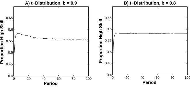
7.1. Auto-regressive Performance. In Section 2, we showed that inefficient selection can happen when performance follows a random walk (Figure 3). The random walk specification assumes that a random draw during the first period of the lifetime of an agent, εi,1, remains relevant during
the lifetime of an agent. In some cases it may be more realistic to assume that the impact ofεi,t
decays over time. This can be modeled by assuming that performance follows an autoregressive structure. Specifically, consider an agent that entered in periodt. Her performance in periodt,pi,t,
0 20 40 60 80 100 0.4
0.45 0.5 0.55 0.6 0.65
Period
Proportion High Skill
A) t−Distribution, b = 0.9
0 20 40 60 80 100
0.4 0.45 0.5 0.55 0.6 0.65
Period
Proportion High Skill
[image:29.612.140.470.122.274.2]B) t−Distribution, b = 0.8
Figure 10. How the proportion of high skill agents changes over time when
per-formance follows an autoregressive process, pi,t+1 =bpi,t+εi,t+1, and A) εi,t are
drawn from a t-distribution with 1 degree of freedom, w= 0.35, andb= 0.9 and B) εi,t are drawn from a t-distribution with 1 degree of freedom, w = 0.35, and b= 0.8. Each graph is based on 10,000 simulations, each with 50 firms, where the
w percent firms with the lowest performances are replaced in every period.
identical to the random walk specification above. Lower values ofbimply lower levels of dependence between performances in consecutive periods (i.e., lower autocorrelation).
Simulations show that the proportion of high skill agents can decline even whenbis lower than 1. To illustrate this, suppose there are 50 agents. Each agent is equally likely to have high (ui= 1)
or low (ui= 0) skill. In each periodt the agents with thew percent lowest performance (pi,t) are
removed from the population. Each eliminated agent is replaced by a new agent. The probability that a new agent has high skill (uj = 1) is 50%. Figure 10 plots how the proportion of high skill
agents changes over time when A)εi,t are drawn from a t-distribution with 1 degree of freedom, w= 0.35, and b= 0.9 B)εi,t are drawn from a t-distribution with 1 degree of freedom, w= 0.35,
and b = 0.8. As shown, the proportion of high skill agents eventually declines in the first case, whenb= 0.9, while the proportion of high skill agents initially increases and then reaches a plateau whenb= 0.8.
0 20 40 60 80 100 −0.5
0 0.5 1 1.5
Period
Average Skill
A) Normal Distribution
0 20 40 60 80 100
−0.5 0 0.5 1 1.5
Period
Average Skill
[image:30.612.139.471.106.257.2]B) t−Distribution
Figure 11. How the average level of skill changes over time when skill is drawn from a normal distribution with mean 0 and variance 1 and the noise term is drawn from A) a normal distribution with mean 0 and variance 1 B) a t-distribution with 1 degree of freedom. Each graph is based on 10,000 simulations, each with 50 firms, where the 10% firms with the lowest performances are replaced in every period.
during the lifetime of a firm. The performance of firm i in period t, pi,t, is equal to the sum of
its capability, ui, and a noise term, εi,t: pi,t = ui +εi. In each period t the 10 percent lowest
performing firms (based onpi,t) are removed from the population. Each eliminated firm is replaced
by a new firm with performancepj,t=uj+εj, whereuj is drawn from a normal distribution with
mean 0 and variance 1 andεjis drawn from densityfε. εj remain the same during the lifetime of a
firm. Figure 11 shows how the average level of skill changes over time (based on 10,000 simulations each withn= 50 firms). Whenfεis a normal distribution with mean 0 and variance 1, the average
level of skill increases over time. Whenfε is a t-distribution with 1 degree of freedom the average
level of skill initially increases but eventually decreases.
The case of a continuous skill distribution is more difficult to handle formally than a binary distribution. What can be demonstrated formally is that whenever the hazard function of the noise distribution is increasing (which is true, for example, for a normal distribution) then average skill increases over time. Formally, suppose that skill (i.e.,ui) is drawn from a distribution with density gu, wheregu can be continuous or discrete. As before, we denote by fε the density of the noise
term and suppose performance equals skill plus the noise term drawn in period 1: pi,t =ui+εi,1.
Theorem 5. If the hazard function of the distribution of the noise term, hε(x), is an increasing
Proof. See Appendix E.
We have not been able to derive necessary or sufficient conditions for when average skill eventually declines. On the basis of simulations, however, we conjecture that average skill eventually decreases if the skill distributiongu has an increasing hazard function (such as the normal) and the noise
distributionfεhas a decreasing or eventually decreasing hazard function (such as the t-distribution
with 1 degree of freedom). By contrast, if the skill distribution gu and the noise distribution fε
both have decreasing hazard functions (for example, they are both t-distributions) then average skill increases over time. The general lesson seems to be that average skill can decrease over time when the noise terms are drawn from a distribution with a ‘longer’ tail than the skill distribution (cf. Denrell & Liu (2012)).
8. When are the results relevant?
Our model shows that the proportion of high skill agents eventually declines as a result of selection when four conditions are satisfied:
(1) The hazard function of the noise distribution is always decreasing (Theorem 2b) or eventu-ally decreasing (Theorem 2c). Theorem 3 also shows that the proportion of high skill agents will converge to 50% ast → ∞ when the distribution of the noise term is ‘long-tailed’, a sub-class of heavy-tailed distributions.
(2) The impact of skill on performance is limited. Theorem 2 assumes that there are only two levels of skill but Figure 11 shows that the average skill also declines over time when skill is drawn from a normal distribution (which is not long-tailed) and the noise term is drawn from a t-distribution (which is long-tailed).
(3) Performance in a given period strongly depends on performance in earlier periods. The-orem 2 assumes that the level of performance remains the same during the lifetime of an agent, but Figure 3 shows that the proportion of high skill agents may also decline over time when the noise term follows a random walk. Figure 10 shows that we can get the same result when performance follows an autoregressive process,pi,t+1 =bpi,t+εi,t+1, as long
asbis sufficiently close to one.
(4) The threshold level of performance required for survival increases over time, as a result of selection based on relative performance.
Consider first the conditions regarding the noise distribution. The concept of a ‘long-tailed’ distribution is perhaps the easier one to understand intuitively. Informally, a distribution is long-tailed if the probability of an extremely high level of performance for an agent with high skill (the probability that 1 +εi > c when c → ∞) is about the same as the probability of an extremely
high level of performance for an agent with low skill (the probability that εi > c when c → ∞).
Intuitively, if the error term is drawn from a long-tailed distribution, then the level of skill has almost no impact on the probability of an extreme event. It follows that an extreme event (a very high level of performance) is not informative about the level of skill of the agent.
Several well-known heavy-tailed distributions are long-tailed, including the Pareto distribution, the Log-normal distribution, and the Cauchy distribution (i.e., the t-distribution with one degree of freedom). Moreover, researchers have shown that these distributions fit several important economic outcomes and social indicators. The Pareto distribution and the Log-normal fit the distribution of wealth. (e.g., the wealth of the top 1% population follows a Pareto distribution whereas the wealth of the rest of the population follow a Log-normal distribution, see Levy & Levy (2003)). Stock-market returns fit a t-distribution (Blattberg and Gonedes, 1974). Our model applies in settings where the performance of an agent equals a skill component plus a random draw from these distributions. Our model does not apply in settings where performance is subject to a noise term drawn from a light-tailed distribution such as the normal distribution.
One setting where our results are relevant is firm size. The firm size distribution fits a Log-normal distribution with an upper Pareto tail (Growiec et al., 2008). Moreover, the empirical evidence suggests that random variation, rather than systematic variation in growth rates, account for most of the variance in firm size (Geroski, 2005; Coad, 2007). This suggests that repeated selection based on firm size (which could occur if there are economies of scale, implying that size strongly impacts performance) can lead to a decline in average firm ‘capability’ over time. Our results also have interesting implications for firm growth rates. Evidence suggests that firm growth rates follow a Laplace distribution (Bottazzi et al., 2001; Bottazzi & Secchi, 2003)3with a low degree of autocorrelation (Coad, 2007). The Laplace distribution is heavy-tailed distribution which is not ‘long-tailed’. Thus, the result that average ‘capability’ may decline as a result of repeated selection does not hold for this distribution. However, the hazard function for the Laplace distribution is eventually constant (see Table 1) and Theorem 2d implies that, for such a noise distribution, the proportion of high skill agents does not increase over time, as a result of repeated selection, but reaches a plateau. This result may be relevant to explaining the puzzling weak association between
productivity and growth (Bottazzi et al., 2001, 2010): repeated selection based on growth will not lead to an increasing proportion of highly productive firms.
The second condition is realistic in settings where variation in skill is limited and unlikely to be responsible for extreme outcomes. Consider trading: it is possible that an individual without skill (e.g., without above average ability to make money in the stock market) might obtain a really high return from trading during one year. Systematic variation in trading ability may exist but explains only a small percentage of the variance in trading results. In other tasks it is inconceivable that low skilled individuals will obtain extremely high outcomes. Consider the 100-meter dash. An unskilled individual who runs 100 meters in 15 seconds, on average, will not, by luck, be able to run below 10 seconds. Many economically relevant tasks are similar: low quality producers will not, by luck, be able to turn out high quality products. Nevertheless, economic outcomes such as profitability, which depend on demand in addition to technical skill, are subject to many uncontrollable factors. For example, demand for cultural products can be very difficult to forecast (Salganik et al., 2006). As a result, it is conceivable that a low-quality producer, who happened to produce what became a fashionable product, would become very profitable.
When are these four conditions applicable to the selection of firms? An example consists in firms producing a product with success subject to strong network externalities. These firms may differ in their research and development capabilities but their level of performance will strongly depend on whether their product became popular early on and generated a large installed base; an outcome which is related to product quality but also depends on many factors beyond the control of management. If product demand is subject to strong network externalities, performance will be subject to a rich-get-richer dynamics (Arthur, 1989; Barabasi & Albert, 1999) that can generate a heavy-tailed distribution of outcomes (Simon, 1955; Barabasi & Albert, 1999). Over time, firms with poor performance will exit the industry and firms with high performance will grow. Eventually the industry will be dominated by one or a few firms with high market shares. Our model implies that the average research and development capabilities of survivors may decline systematically over time, after an initial increase (compare Figure 9).
When are the four conditions be applicable to selection of individuals within organizations? Se-lection among individuals in academia provides a possible illustration. Academics are evaluated for jobs, tenure, and chairs based primarily on their research output such as high prestige publications, impact, and citations. Both the number of publications and citations follow heavy-tailed distribu-tions such as the Pareto and the Log-normal (Radicchi et al., 2008). Research on the Matthew Effect suggests that evaluation in academia is noisy and good luck can have a persistent impact because good performance leads to increased attention and resources and improves the chances of high subsequent performance (Merton, 1968). Performance is also persistent because both the num-ber of publications and citations are added up throughout a career. Finally, advancement within schools and to universities of higher status often depends on performance relative to peers. Overall, these observations suggest that it is possible that average research skills decreases over time, as academics are subject to more and more selections.