MODELLING OF DAILY ACTIVITY SCHEDULE OF WORKERS
USING UNSUPERVISED MACHINE LEARNING TECHNIQUE
Anu P. Alex1, Manju V. Saraswathy2, Kuncheria P. Isaac3 1, 2 The College of Engineering Trivandrum, Kerala, India
3 APJ Abdul Kalam Technological University Kerala, India
Received 13 November 2015; accepted 12 February 2016
Abstract: Travel demand models are used to replicate the real world travel demand and to predict the future travel demand. A behavioural oriented approach in travel demand analysis is provided by activity based travel demand modelling and it provides a better understanding of the travel behaviour of an individual. A sequential modelling approach using econometric models is commonly used in activity based travel modelling. In this method, error obtained in one model will be carried forward to the second model and so on. Hence chances of accumulation of error are more at the final stage, when the models are used for prediction. Hence an attempt is made in this study to replace the sequential econometric modelling approach with simultaneous modelling approach using an unsupervised machine learning technique. Three stage Neural Network modelling used in this study replaces sixteen stage econometric models. The predictive accuracy of all the output parameters was compared in both the modelling approaches. Results shows that Artificial Neural Network (ANN) results outperform econometric models. The decrease in percentage error ranges from 2.22% to 27.17%.
Keywords:work activity, ANN, econometric models.
1 Corresponding author: [email protected]
1. Introduction
Travel demand modelling is an essential tool in transportation planning. Traditional trip based travel demand models are successfully replaced by superior and advanced activity based travel demand modelling in various countries. This is due to its capability in modelling the time and sequence of activities as well as the competence of incorporating the behaviour of individuals. Activity based travel demand models are based on the renowned notion that ‘travel is derived from demand to pursue in activities’. Travel or trips are emerged as a result of activity participation process. Researchers often explore activities from a variety of perspectives. Damm (1980)
The most comprehensive and the only operational computational process model is ALBATROSS developed by Arentze and Timmermans (2000). It is a rule-based system that predicts activity patterns. Bhat and Singh (2000) and Bhat et al. (2004) developed an econometric model called Comprehensive Econometric Micro-simulator for Daily Activity-travel Patterns (CEMDEP), in which a comprehensive activity generation-allocation scheduling model was proposed. It considered ‘work/ school’ as the primary activity of the activity patterns. For prediction of the work/ school duration, it used an econometric hazard model with covariates as socio demographics and work characteristics. By developing FAMOS (Florida Activity Mobility Simulator) Pendyala et al. (2005) proposed a prism constrained simulation approach where work/school are considered to be fixed activities within the daily activity schedule. Roorda et al. (2008) developed a rule-based activity scheduler; TASHA, which also takes the same approach for generating work/ school duration. Eluru et al. (2010) developed a continuous time activity-based microsimulation model of travel demand for the Southern California Association of Governments.
Muralidhar et al. (2006) developed a prototype of time-space diary design which would be user friendly, offers less burden on respondent, and ensures good quality and quantity of data. The study proved that time-space diary has a better performance than conventional travel diary format. Surekha (2009) developed a microsimulation model for activity travel pattern for Tiruchirappalli City, Tamil Nadu, India. Muralidhar et al. (2005) presented a tour-based approach of modelling mode choice of the residents of Mumbai city of India. The study focused on
the development of mixed logit model and it is compared to Multinomial Logit Model (MNL). It was found that the performance of the mixed logit model is better than MNL. Sreela et al. (2013) studied the shopping activity travel behaviour of workers in Calicut city, one of the major urban centres in Kerala. This study revealed that the age of the person and household income positively influence the participation in shopping activity, while travel distance and number of non- working adults in household negatively influence shopping. Manoj and Verma (2013) studied the activity-travel behaviour of non-workers in Bangalore city of India. This study modelled the out-home activity participation behaviour of non-workers using a primary activity-travel survey data. Vishnu and Srinivasan (2013) used tours as the fundamental unit of analysis to study the discontinuity in mode choice and independence assumption in trip-based models. The nominal nature of the dependent variable is captured using MNL model.
unsupervised machine learning technique, Artificial Neural Network, in which a sixteen stage econometric models are replaced with three stage ANN networks. The predictive accuracy of all the output parameters was compared in both the modelling approaches. The study concentrated on the daily activity generation and scheduling of workers.
2. Methodology and Data Description
T h e s t u d y a r e a s e l e c t e d i s Thiruvananthapuram City, the capital of Kerala, lying in the southernmost part of India. As per 2011 census data, Thiruvananthapuram city consists of 2,42,149 households with a total population of 9,66,856. To develop the daily work generation and scheduling model system, an activity travel diary was designed and data were collected via home interview survey by random selection of households. The study used the travel time diary of 9530 members collected from 2521 households. Among this, the working population is 41%, of which, 51% are male and 49% are female. Daily work and other activity scheduling models were developed using 80% of the collected data and the rest 20% were used for validation. In order to develop the conventional activity based models, an econometric approach used in CEMDAP (Bhat and Singh, 2000) was adopted, in which daily activity schedule models consist of work and other activity
generation and scheduling models. Work generation models involve model for finding the out-home work activities and duration and start time of daily work activity. Work scheduling models involve duration and mode of commute before and after work, probability to participate in other activities, duration, time of occurrence and mode of other activities, probability and duration of stop during commute and home stay duration between the out home activities. Econometric models and ANN models were developed in the present study to predict all the above response variables. These models were then validated and prediction accuracies of all the models were compared.
3. Econometric Modelling Approach
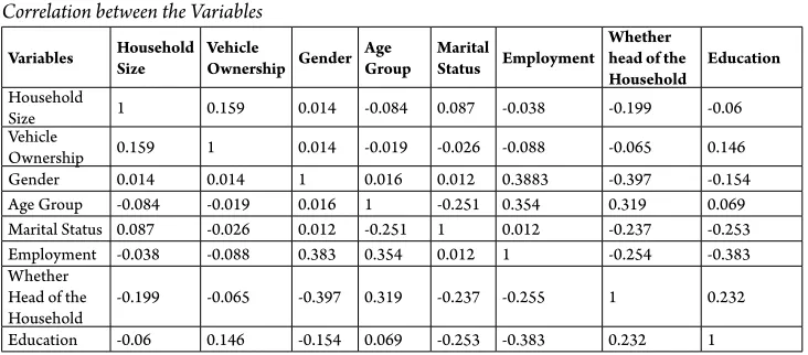
Using econometric or discrete choice modelling approach, sixteen discrete choice models were developed. This includes eight models for predicting work activity generation and scheduling, four models for other activity of workers and four models for stop level pattern of workers during commute. The independent variables used and their coding are given in Table 1. The correlation coefficients between the variables are given in Table 2. It can be observed from the table that the correlation coefficients between all the variables are less than 0.5 which indicates that the variables are not correlated to each other.
Table 1
Coding of Variables Used
Independent Variables Category
Household size 1 to 8
Vehicle Ownership No vehicle-1, Only Two Wheeler-2, Only Car-3, Both TW and car or more than one car-4 Gender Male-1, Female-2
Age Group “18-25”-1, “26-40”-2, “41-55”-3, “56-70”-4 Marital Status Married-1, Unmarried-2
Employment Government sector-1, Private sector-2, Self employed-3 Mode of Commute Walk / Cycle-1, TW-2, Car-3, Bus-4, Train-5 Relationship Household Head-1, Other-2
Table 2
Correlationbetween the Variables
Variables Household Size Vehicle Ownership Gender Age Group Marital Status Employment Whether head of the
Household Education
Household
Size 1 0.159 0.014 -0.084 0.087 -0.038 -0.199 -0.06 Vehicle
Ownership 0.159 1 0.014 -0.019 -0.026 -0.088 -0.065 0.146 Gender 0.014 0.014 1 0.016 0.012 0.3883 -0.397 -0.154 Age Group -0.084 -0.019 0.016 1 -0.251 0.354 0.319 0.069 Marital Status 0.087 -0.026 0.012 -0.251 1 0.012 -0.237 -0.253 Employment -0.038 -0.088 0.383 0.354 0.012 1 -0.254 -0.383 Whether
Head of the
Household -0.199 -0.065 -0.397 0.319 -0.237 -0.255 1 0.232 Education -0.06 0.146 -0.154 0.069 -0.253 -0.383 0.232 1
3.1. Work Activity Generation and
Scheduling
Work activity generation part includes models for finding the out-home work activities, how long the individual spend for work and when he/she starts the work i.e.: daily work duration and daily work start time, and finally the duration of commute before and after work activity. The first part is developed using binary logit model since the dependent variable is dichotomous. i.e.; outcome of the model expects the probability of yes/no for an individual to go for out-home work activity. MLR is used for predicting duration or time. Coefficients of the attributes in different models are given in Tables 3 and 4.
Model 1 given in Table 3 shows that the significant factors which cause an individual to be an out-home worker are household size, gender, age group, marital status, whether the person is head of the household and employment. Work start time is modelled as the time of first arrival at the work. The influencing factors of daily work start time are gender, age group, education and daily
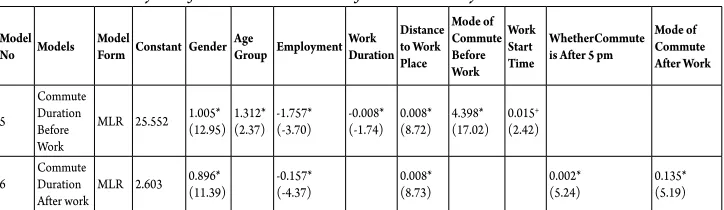
The commute duration of a person from home to work place before and after work are also modelled as MLR (Model 5 and 6). The significant variables are found to be vehicle ownership, duration of work activity, employment, mode of commute, age group, gender and start time of work. It is seen that self-employed people take less time for their commute before work, probably because their working place is in the vicinity of their
residential areas. If the working duration is more, commute duration is less. This is due to the fact that people stay near the working place, if the working duration is more. As the mode of commute changes from walk or cycle to train, commute duration decreases. Older people take long time for commute compared to younger people. Females are observed to take more commute time than males.
Table 3
Econometric Model System for Work Activity Generation
Model
No Models ModelForm ConstantHousehold Size Gender Age Group Marital Status Employment Education Person is Head of the Household
Work Duration
1 Out-home Work Activity
Binary
Logit 14.199 0.195*(3.19) -1.129*(-6.29) 0.923*(12.00) -3.087*(-13.66)-3.713*(-28.52) 1.390*(7.27)
2 Work Duration MLR 530.402 -36.694*(-6.92) -8.671(-2.52)+ 24.033*(11.26) -20.470*(-5.97)
3 Work Start Time MLR 519.862 -21.598*(-6.55) -4.021(-2.15)+ 8.248*(4.02) -0.248*(-17.65)
4 Distance to Work
Place MLR 36.285
-4.999*
(-3.01) -2.994*(-3.00) 3.681 +
(2.08) -3.520*(-4.41) -0.020*(-2.85)
*Variables at 1% level of significance +Variables at 5% level of significance ( ) Values in brackets are t statistics
Table 4
Econometric Model System for Commute Duration for Work Activity
Model
No Models ModelForm Constant GenderAge Group EmploymentWork Duration Distance to Work Place
Mode of Commute Before Work
Work Start Time
WhetherCommute is After 5 pm
Mode of Commute After Work
5
Commute Duration Before Work
MLR 25.552 1.005*(12.95) 1.312*(2.37) -1.757*(-3.70) -0.008*(-1.74) 0.008*(8.72) 4.398*(17.02) 0.015(2.42)+
6 Commute Duration
After work MLR 2.603 0.896*
(11.39) -0.157*(-4.37) 0.008*(8.73) 0.002*(5.24) 0.135*(5.19)
Table 5
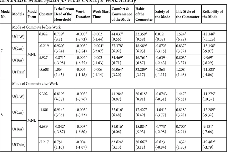
Econometric Model System for Mode Choice for Work Activity Model
No Models Model Form Constant
Is the Person Head of the Household
Work
DurationWork Start Time Comfort & Convenience of the Mode
Habit of the Commuter
Safety of
the Mode Life Style of the Commuter Reliability of the Mode
7
Mode of Commute before Work
U(TW)
MNL
6.022 0.719*
(3.5) -0.003*(-3.73) -0.002(-1.44) 44.837*(9.56) 22.359*(9.58) 0.012(0.05) 1.524*(6.95) -12.346*(-11.23)
U(Car) -0.219 0.920*(3.94) -0.003*(-3.54) -0.004*(-2.87) (6.92)37.378* 18.589*(6.93) -0.872*(-3.15) 0.837*(3.37) -13.158*(-9.97)
U(Bus) 5.927 -0.871*(-3.95) -0.006*(-6.55) -0.002(-1.63) (6.71)34.469* 16.761*(6.57) -0.639+(-2.43) 0.805*(3.37) -9.969*(-8.29)
U(Train) -5.608 1.064(1.45) -0.004(-1.18) -0.006(-1.14) (3.20)66.064* 32.209*(3.17) -0.863(-1.11) 1.208(1.46) -21.583*(-4.06)
8
Mode of Commute after Work
U(TW)
MNL
5.302 0.819*
(4.05) -0.003*(-3.76) 41.284*(8.87) 20.615*(8.91) -0.0743(-0.31) 1.447*(6.63) -11.275*(10.37)
U(Car) -1.801 0.914*(3.96) -0.003*(-3.22) 35.016*(6.48) 17.427*(6.49) -1.041*(-3.77) 0.815*(3.28) -12.289*(-9.32)
U(Bus) 4.689 -0.842*(-3.87) -0.005*(-6.60) 31.016*(6.06) 15.084*(5.93) -0.773*(-2.98) 0.700*(2.94) -9.181*(-7.66)
U(Train) -7.217 0.751(1.10) -0.004(-1.07) 62.624*(3.13) 30.667*(3.12) -0.623(-0.84) 1.432(1.80)+ -19.462*(-3.79)
*Variables at 1% level of significance +Variables at 5% level of significance ( ) Values in brackets are t statistics
3.2. Other Activity of Workers
Models developed for other activity of workers include probability to participate in other activities, time of occurrence, mode used and duration of other activities. The coefficients of various influencing attributes in all the models are given in Table 6-8. Probability to participate in other activities such as personal business and recreation, shopping and eat out are modelled using MNL (Model 9). The influencing factors for participation in personal business and recreation are gender, marital status, work duration, vehicle ownership and household size. It is observed from the model that males and married persons are more involved in personal business and recreation than females. As work duration increases and vehicle
ownership decreases there is less probability to involve in this activity. Probability of shopping depends on household size and work duration. As household size increases and work duration decreases there is more probability of shopping of workers. Males, younger and unmarried people involve more in eat out activity. Gender, age group, marital status and work duration are the influencing factors of eat out activity of workers.
ownership. It is found that unmarried people prefer to go for other activity after work or during work. As the work duration increases, probability to go for other activity after work decreases and during work increases. As the starting time of work increases, probability of other activity after work and during work decreases than before work. When the vehicle ownership increases, probability of other activity after work increases.
Modes of other activities were identified as walk/cycle/auto, two wheeler, car and bus. The choice of mode for other activity was also modelled with MNL with walk/cycle/auto as the base value and is given in Model 11. Utility of TW are positively influenced by purpose and time of occurrence of activity. Utility of car is positively influenced by gender, age group, purpose and time of occurrence of activity and vehicle ownership. Purpose of activity positively influences and vehicle ownership negatively influences the utility of bus.
Duration of other activity was modelled as MLR as shown in Model 12. The influencing factors are work duration, purpose and mode of activity. Individuals spend more time for personal business and recreation than shopping followed by eat out. It is observed that as work duration increases, duration of other activity decreases and when mode used for the activity changes from walk to bus, duration also increases.
3.3. Stop Level Pattern during other
Activity
While commuting before and after work, the worker may stop for other activities and it is modelled in this section. Stratification of the collected data is such that about 91.19% of the workers are not stopping during commute, 7.89% stop during after work
commute and only 0.92% stop before work commute. Hence the stop level pattern of workers during after work commute is only modelled. The models include probability to stop for other activity, purpose of stop and duration of stop. The coefficients of the models are shown in Table 9. Probability to stop is modelled as binary logit as given in Model 13. Model shows that females and married people have more probability to stop during after work commute. If the mode of commute is bus, lesser the probability to stop and if the commute duration and distance are more, there is higher probability to stop.
Purpose of stop during commute after work are identified as care for children/spouse/ elderly, shopping and personal business and recreation. It is modelled as MNL and with base value as ‘care for children/spouse/ elderly’. It is given in Model 14. It is observed that there is more probability for care for children/spouse/elderly than shopping and personal business when the commute duration after work is more. This will be more than shopping if the household size increases. There is more probability of personal business and recreation during commute after work for self employed persons.
Duration of stop is modelled as MLR as shown in Model 15. Model shows that the influencing factors are commute duration after work, distance and purpose of stop. If the commute duration and distance increases, duration of stop will be less. Duration of stop for care for children/ spouse/elderly is less than that of shopping followed by personal business and recreation.
are given in Table 10. It shows that home stay duration will be less for other activity after work than that before work. If the person reaches the work place by late, obviously home stay duration will be more. If the commute
duration and work duration are more home stay duration will be less and as the vehicle ownership increases home stay duration also increases. Females and married people stay more at home between the activities.
Table 6
Econometric Model System for other Activity Generation of Workers
Model
No. Models Model Constant Household Size Gender Age Group Marital Status Work Duration Vehicle Ownership
9 Probability of Other Activity U(Personal
Business & Recreation)
MNL
1.264 -0.183*(-3.53) -1.520*
(-9.24) 0.007(0.08) -0.804*(-4.66) -0.001 +
(2.14) 0.130*(2.59)
U(Shopping) -1.641 0.130(1.75)+ -0.264(-1.35) 0.198(1.63) -0.446(-1.59) -0.002(-2.18)+ -0.016(-0.20)
U(Eat out) -6.624 0.081(0.94) -1.281*(-3.76) -0.324(-2.37)+ 0.725*(2.88) 0.006*(7.75) 0.111(1.22)
*Variables at 1% level of significance +Variables at 5% level of significance ( ) Values in brackets are t statistics
Table 7
Econometric Model for Time of Occurrence of other Activity Workers
Model
No. Models Model Constant Marital Status Employment Work duration Purpose of Activity Work Start Time Vehicle ownership
10 Time of Occurrence of Other Activity U(After
work) MNL 11.315 0.998*(3.14) -0.067(-0.57) -0.011*(-7.79) 2.216*(12.50) -0.021*(-7.92) 0.205 + (1.80) U (work
based) MNL -4.811 1.681*(5.29) 0.375*(3.13) 0.004*(2.94) 2.001*(10.62) -0.008*(-3.52) 0.126(1.10) *Variables at 1% level of significance +Variables at 5% level of significance ( ) Values in brackets are t statistics
Table 8
Econometric Model System for Mode and Duration of other Activity of Workers
Model
No. Models Model Constant Gender Age Group Work Duration Purpose of Activity Time of Occurrence of activity
Vehicle
Ownership Mode of Activity
11 Mode of Other Activity
U( TW) MNL -2.523 -0.481(-1.55) -0.172(-1.28) 0.941*(7.53) 0.848*(6.54) 0.132(1.41)
U(Car) -9.364 0.773*(2.13) 0.578*(3.07) 0.887*(4.79) 0.906*(4.57) 0.664*(4.07)
U(Bus) -6.205 1.193(1.41) -0.544(-0.82) 1.982(-2.88)+ 0.575(0.79) -1.043(-2.03)+
12 Duration of other
Activity MLR 108.664
-0.049*
(-2.3) -22.938*(-8.06) 7.652 + (2.76)
Table 9
Econometric Model System for Stop Level during other Activity of Workers
Model
No. Models Model Constant Gender Marital Status
Mode of Commute After Work
After work Commute
Duration Distance Household Size Employment Purpose of Stop
13 Probability of stop during Commute After work
Binary
logit -3.629 0.501
+
(2.51) -0.738
+
(-2.51) -0.206*(-3.48) 0.057*(15.44) 0.132*(-7.23) 14 Purpose of Stop during Commute After work
U(Stop=shopping) MNL 0.488 -0.051*(-4.03) -0.463(-2.48)+ 0.282(0.92) U(Stop=Personal
business and
recreation) MNL -8.732
-0.094*
(-5.67) -0.402(-1.31) 1.341 *(2.93)
15 Duration of stop during after work
commute MLR -8.523
-0.493*
(-12.31) -0.746*(-3.62) 13.659*(3.84)
*Variables at 1% level of significance +Variables at 5% level of significance ( ) Values in brackets are t statistics
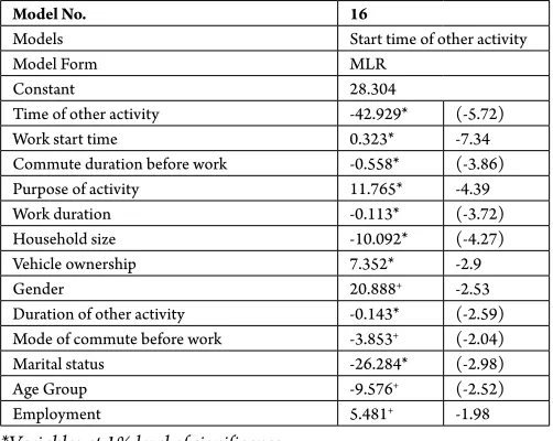
Table 10
Econometric Model for Start Time or other Activity
Model No. 16
Models Start time of other activity
Model Form MLR
Constant 28.304
Time of other activity -42.929* (-5.72)
Work start time 0.323* -7.34
Commute duration before work -0.558* (-3.86) Purpose of activity 11.765* -4.39
Work duration -0.113* (-3.72)
Household size -10.092* (-4.27)
Vehicle ownership 7.352* -2.9
Gender 20.888+ -2.53
Duration of other activity -0.143* (-2.59) Mode of commute before work -3.853+ (-2.04)
Marital status -26.284* (-2.98)
Age Group -9.576+ (-2.52)
Employment 5.481+ -1.98
*Variables at 1% level of significance +Variables at 5% level of significance ( ) Values in brackets are t statistics
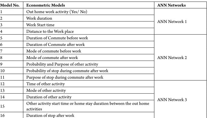
4. Neural Network Modelling
Artificial Neural Network as a computing system is made up of a number of simple,
most popular of the much architecture currently available, was used in this study. The network was trained using an error back propagation training algorithm. This algorithm adjusts the connection weights according to the back propagated error computed between the observed and the estimated results. This is an unsupervised
learning procedure that attempts to minimise the error between the desired and the predicted outputs. The networks used in this study consisted of four layers: one input layer, two hidden layers and one output layer. The sixteen stage econometric models were replaced with three stage neural networks as shown in Table 11.
Table 11
ANN Networks
Model No. Econometric Models ANN Networks
1 Out home work activity (Yes/ No)
ANN Network 1 2 Work duration
3 Work Start time 4 Distance to the Work place 5 Duration of Commute before work
ANN Network 2 6 Duration of Commute after work
7 Mode of commute before work 8 Mode of commute after work
9 Probability and Purpose of other activity 10 Probability of stop during commute after work 11 Purpose of stop during commute after work 12 Time of other activity
ANN Network 3 13 Mode of other activity
14 Duration of other activity
15 Other activity start time or home stay duration between the out home activities 16 Duration of stop after work
First net work was for work activ it y generation, second network for work activity scheduling and third network for other activity of workers. Each network is discussed in detail in the following sections.
4.1. Neural Network for Work Activity
Generation
This network consisted of four layers: one input layer of eight neurons (one for each input variable), two hidden layers of twenty
Fig. 1.
Neural Network for Work Activity Generation
Fig. 2.
Training Performance of Neural Network for Work Activity Generation
4.2. Neural Network for Work Activity
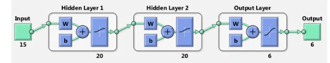
Scheduling
This network also consists of four layers: one input layer of fifteen neurons as input variables, two hidden layers of twenty neurons and one output layer of six neurons as the output variables (Fig. 3). The input variables used are gender, age group, education, marital status, employment, vehicle ownership, whether
the individual is head of the household, work duration, work start time, distance to work place from home, comfort and convenience of the mode, habit of the commuter, safety of the mode, life style of the commuter and reliability of the mode. The output variables are commute mode and duration before and after work, purpose of stop and other activity of workers. The network shows best training performance at 418 epochs (Fig. 4).
Fig. 3.
Fig. 4.
Training Performance of Neural Network for Work Activity Scheduling
4.3. Neural Network for other Activity
of Workers
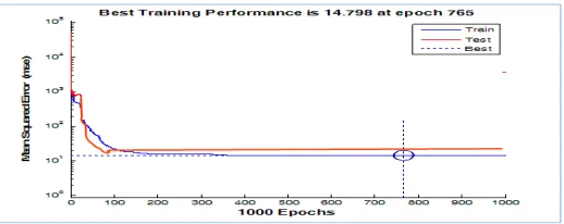
This network was developed with four layers: one input layer of fifteen neurons as input variables, two hidden layers of twenty neurons and one output layer of five neurons as the output variables (Fig. 5). The input variables used are gender, age group, education, marital status, employment, vehicle ownership, whether the individual is head of the
household, work duration, work start time, distance to work place from home, mode and duration of commute before and after work, purpose of other activity and purpose of stop during commute. The output variables are mode of commute, time of occurrence and duration of other activity, duration of stop during commute and duration of home stay between the activities of workers. The best training performance of the network was observed at 765 epoch (Fig. 6).
Fig. 5.
Neural Network for other Activity of Workers
Fig. 6.
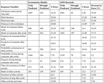
5. Validation of the Models
The models discussed in the previous sections can be used for finding out the generation of work and other activity of workers, timing of out home activities and the mode used for each activity of each individual. Both econometric and neural network models were applied to 20% of the collected data. Results of response variables for each individual were compared between
both approaches. The response variables obtained for MNL and Binary logit models were compared as truly predicted and wrongly predicted and the percentage error is calculated. Response variables obtained from MLR models are compared with the observed values and Relative Root Mean Square Error (RRMSE) was calculated. Percentage errors of all the output variables in both models were also compared. Results are shown in Table 12.
Table 12
Comparison of the Models
Econometric Models ANN Networks
Response Variables Truly Predicted Wrongly Predicted % Error Truly Predicted Wrongly Predicted % Error Decrease in Error (%)
Out home work activity
(Yes/No) 1667 239 12.54 1861 45 2.36 10.18
Work duration 25.84 13.38 12.46
Work start time 22.71 7.27 15.44
Distance to the work place 18.96 11.89 7.07
Mode of commute before
work 940 448 32.29 1192 196 14.1 18.19
Mode of commute after work 955 433 31.19 1201 187 13.48 17.71 Duration of commute before
work 31.74 14.03 17.71
Duration of commute after
work 35.01 16.86 18.15
Probability and purpose of
other activity 992 396 28.53 1133 255 18.34 10.19
Probability of stop during
commute after work 1284 104 7.52 1318 70 5.02 2.5
Purpose of stop during
commute after work 172 19 10.00 176 15 7.78 2.22
Time of occurrence of other
activity 274 126 31.52 359 41 10.33 21.19
Mode of other activity 241 159 39.67 350 50 12.5 27.17
Duration of other activity 22.1 6.18 15.92
Duration of stop after work 22.12 7.12 15
Other activity start time 12.89 5.84 7.05
It can be seen that the accuracy of all the ANN models are greater than econometric models. This is due to the learning ability of ANN compared to the econometric models.
ideal methods for arriving at solutions while defining computing functions or distributions. It takes data samples rather than entire data sets to arrive at solutions, which saves both time and money.
6. Conclusion
Travel demand models are used to replicate the real world transportation system and to predict the future travel demand. A behavioural oriented approach in travel demand analysis is provided by activity based travel demand modelling and it provides a better understanding of the travel behaviour of an individual, but they are very complex and demand more data. The main application of this approach lies in the traffic control policies. The activity travel demand models can vary depending upon the type of data as well as the purpose of the study. There are so many activity generation model systems for developed countries, which are partially and fully operationalized. For a developing country like India, activity based planning process is still at the infant stage due to its complexity and lack of readily available micro data of individuals.
This study is concentrated on the important part of the activity based travel demand modelling, which is daily work activity generation. Thiruvananthapuram, which is the capital city of Kerala in India is selected as the study area for developing the models. A daily activity schedule model system for workers was developed in this study based on two approaches. The first approach was conventional econometric modelling which is sequential modelling. The second approach was ANN modelling, which is simultaneous modelling. Sixteen stage econometric models were replaced
with three stage ANN models in this study. Hence the error accumulation in sequential modelling approach is reduced in this new simultaneous modelling approach. Models in both approaches were validated using 20% of the data and the percentage error was calculated for both approaches. It is seen that ANN models are more predictive than discrete choice models. The decrease in percentage error ranges from 2.22% to 27.17% in the case of ANN models. Hence it can be concluded that the conventional econometric models if replaced with ANN models in activity based modelling will provide better results.
Acknowledgement
The authors are grateful to Kerala State Council for Science Technology and Environment (KSCSTE) for funding the project.
References
Arentze, T.A.; Timmermans, H. 2000. ALBATROSS - A learning based transportation oriented simulation system. In Proceedings of the TRB Conference 2000, USA, Issue No. 1706, 136-144.
Bhat, C.R.; Guo, J.Y.; Srinivasan, S.; Sivakumar, A. 2004. Comprehensive Econometric Microsimulator for Daily Activity-Travel Patterns, TransportationResearch Record:
Journal of the Transportation Research Board, No. 1894, TRB,
National Research Council, Washington, D.C., 57-66.
Bhat, C.R.; Singh, S.K. 2000. A Comprehensive Daily Activity-Travel Generation Model System for Workers,
Transportation Research Part A: Policy and Practice, 34(1):
1-22.
Damm, D. 1980. Interdependencies in activity behavior,
Eluru, N.; Pinjari, A.R.; Pendyala, R.M.; Bhat, C.R. 2010. An econometric Multi-Dimensional Choice Model of Activity-Travel Behaviour, Transportation Letters:
The International Journal of Transportation Research, 2(4):
217-230.
Kitamura, R. 1988. An evaluation of activity-based travel analysis, Transportation,15(1): 9-34.
Manoj, M.; Verma, A. 2013. Analysis and Modelling of Activity-Travel Behaviour of Nonworkersfrom a City of Developing Country, India. In Proceedings of the 2nd Conference of Transportation Research Group of India (2nd
CTRG), Procedia - Social and Behavioral Sciences, 104(2013):
621-629.
Muralidhar, B.; Mathew, T.V.; Dhingra, S.L. 2005. Development of a Mixed Logit Model to Tour Mode Choice for an Urban Region. In Proceedings of International
Conference CUPUM 2005, London U.K.
Muralidhar, B.; Mathew, T.V.; Dhingra, S.L. 2006. Prototype Time-Space Diary Design and Administration for a Developing Country, Journal of Transportation
Engineering, ASCE, 132(6): 489-498.
Pendyala, R.M.; Kitamura, R.; Kikuchi, A.; Yamamoto, T.; Fujii, S. 2005. Florida Activity Mobility Simulator - Overview and Preliminary Validation Results,
Transportation Research Record: Journal of the Transportation
Research Board, No. 1921, Transportation Research Board
of the National Academies, Washington, D.C., 123-130.
Recker, W.W.; McNally, M.G.; Root, G.S. 1986. A model of complex travel behaviour: part I - theoretical development, Transportation Research Part A, 20A(4): 307-318.
Roorda, M.J.; Miller, E.J. 2003. A Prototype Model of Household Activity/Travel Scheduling. Presented at the
Transportation Research Board Annual Meeting.
Roorda, M.J.; Miller, E.J.; Habib, K.M.N. 2008. Validation of TASHA: A 24-h activity scheduling microsilulation model, Transportation Research Part A, 42(2): 360-375.
Saw, K.; Katti, B.K.; Joshi, G.K. 2015. AB temporal trip generation modelling for primary activities: a case study of fast growing metropolitan city, International Journal
for Traffic and Transport Engineering, 2015, 5(2): 120-133.
Sreela, P.K.; Melayil, S.; Anjaneyulu, M.V.L.R. 2013. Modeling of Shopping Participation and Duration of Workers in Calicu. In Proceedings of the 2nd Conference of Transportation Research Group of India (2nd CTRG), Procedia
- Social and Behavioral Sciences, 104(2013): 543-552.
Surekha, N. 2009. Microsimulation of Activity-Travel
Pattern for Tiruchirappalli City, M. Tech Thesis at NIT
Tiruchirappalli.
Vishnu, B.; Srinivasan, K.K. 2013. Tour-based departure time models for work and non-work tours ofworkers. In
Proceedings of the 2nd Conference of Transportation Research Group of India (2nd CTRG), Procedia - Social and Behavioral