www.nat-hazards-earth-syst-sci.net/15/671/2015/ doi:10.5194/nhess-15-671-2015
© Author(s) 2015. CC Attribution 3.0 License.
Modelling rapid mass movements using the shallow water equations
in Cartesian coordinates
S. Hergarten1and J. Robl2
1Universität Freiburg i. Br., Institut für Geo- und Umweltnaturwissenschaften, Freiburg, Germany 2Universität Salzburg, Fachbereich Geographie und Geologie, Salzburg, Austria
Correspondence to: J. Robl ([email protected])
Received: 29 September 2014 – Published in Nat. Hazards Earth Syst. Sci. Discuss.: 4 November 2014 Revised: – – Accepted: 11 March 2015 – Published: 30 March 2015
Abstract. We propose a new method to model rapid mass movements on complex topography using the shallow wa-ter equations in Cartesian coordinates. These equations are the widely used standard approximation for the flow of wa-ter in rivers and shallow lakes, but the main prerequisite for their application – an almost horizontal fluid table – is in general not satisfied for avalanches and debris flows in steep terrain. Therefore, we have developed appropriate cor-rection terms for large topographic gradients. In this study we present the mathematical formulation of these correc-tion terms and their implementacorrec-tion in the open-source flow solver GERRIS. This novel approach is evaluated by sim-ulating avalanches on synthetic and finally natural topogra-phies and the widely used Voellmy flow resistance law. Test-ing the results against analytical solutions and the proprietary avalanche model RAMMS, we found a very good agree-ment. As the GERRIS flow solver is freely available and open source, it can be easily extended by additional fluid models or source areas, making this model suitable for simulating sev-eral types of rapid mass movements. It therefore provides a valuable tool for assisting regional-scale natural hazard stud-ies.
1 Introduction
Rapid mass movements such as avalanches, debris flows, and lahars are globally abundant surface processes in steep mountainous areas characterized by high process veloci-ties and large masses of granular material involved (e.g. Kirschbaum et al., 2010). Therefore, rapid mass movements represent first-order threats whenever their process domains
intersect with populated areas and infrastructure for trans-port (streets, railway lines), energy supply (power plants, pipelines, electricity lines), or tourism (e.g. ski resorts). While most of the villages prone to rapid mass movements have already implemented hazard mitigation strategies by a combination of permanent and temporal preventive mea-sures, the latter are progressively developed in remote moun-tainous regions where historical records on rapid mass move-ments are sparse, so that the level of threat is ambiguous. In combination with field mapping and remote sensing, numer-ical models describing the motion of granular material on general topography are the primary tool to evaluate the po-tential impact of rapid mass movements on infrastructure in these remote places. Run-out distance, flow and depositional depth, velocity, and momentum of a granular flow resulting from physically based numerical models represent key pa-rameters to (a) delineate hazard zones on the regional scale, (b) locate ideal corridors and construction areas for new in-frastructure, and (c) develop mitigation strategies for protect-ing planned and already existprotect-ing infrastructure against these natural hazards (Hsu et al., 2010; Keiler et al., 2006). To ful-fill these tasks, codes have to be equipped with advanced nu-merical techniques to reach the required computational per-formance (e.g. adaptive mesh refinement), have to provide an interface to geographic information systems (GIS) and should be controllable by a scripting language to perform Monte Carlo simulations and parameter studies for entire val-leys and hundreds of process domains.
The implementation of a new rheology model even in open-source scientific codes by the user is in general not practica-ble, because a deep knowledge on the specific code and fluid dynamics is required. Other recent codes such as Flow-R (Horton et al., 2013) replace the equations of continuum me-chanics by more empirical, grid-based algorithms and thus require a higher degree of calibration.
The Voellmy rheology (Voellmy, 1955) is frequently used to describe debris flows and dense snow avalanches and is implemented in proprietary software products such as RAMMS (Christen et al., 2010), SAMOS-AT (Sampl and Zwinger, 2004; Sailer et al., 2008; Granig and Jörg, 2012), and ELBA+. The latter has been extensively used by the Austrian avalanche and torrent control, but peer-reviewed publications on technical details are still missing. Aston-ishingly, there are no open-source codes that fulfill all re-quirements mentioned above to describe granular flow with a Voellmy rheological model on complex topography. How-ever, there are several open-source packages for a wide range of fluid dynamical problems that provide state-of-the-art flow solvers and a variety of numerical accessories like automatic meshing routines or adaptive mesh refine-ment, such as OPENFOAM (Weller and Weller, 2008, http: //www.openfoam.com), CLAWPACK (LeVeque et al., 2011; Berger et al., 2011, http://clawpack.github.io), and GERRIS (Popinet, 2009, http://gfs.sourceforge.net). Besides many other applications, these codes are routinely used to predict the propagation of tsunamis in ocean basins (Popinet, 2012) or to model the extent of inundation areas during flooding (An and Yu, 2012) by solving the nonlinear shallow water equations being the standard approximation for the flow of water in rivers and shallow lakes. These numerical packages are operated by highly flexible parameter files that allow the implementation of new fluid rheology models without writ-ing additional source code, so that it is temptwrit-ing to describe rapid mass movements with one of these fluid dynamics soft-ware packages.
In this spirit, two-dimensional models for rapid mass movements on a given topography are similar to the shal-low water equations. In both concepts, vertically averaged velocities are considered, and the rheology of the medium and effects of turbulence are taken into account in form of a friction term depending on flow depth and velocity. However, the widely used shallow water equations are only applicable if the water table is almost horizontal. This condition is in general not satisfied for mass movements in steep terrain, so that more elaborate approaches are required here.
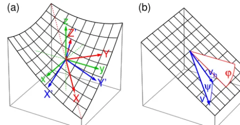
These approaches can be subdivided into two major classes according to the coordinate system used. The differ-ent coordinate systems are illustrated in Fig. 1a for the ex-ample of a channel not parallel to any of the Cartesian coor-dinate axesx,y, andz. The first group of models focuses on flow in a given channel and uses a curvilinear coordinate sys-tem with azaxis being always normal to the surface, while thexcoordinate follows the so-called thalweg in downslope
y x
z
Y
X Z’
Y’ X’
(a) (b)
v vh
ψ ϕ
Figure 1. (a) Different coordinate systems used for modelling mass movements in a channel not parallel to any of the Cartesian coor-dinate axes. Green: Cartesian coorcoor-dinatesx,y, andz(this study). Blue: Coordinates aligned to the surface (x0 andy0parallel to the surface,z0normal to the surface). Red: Coordinates aligned to the surface (x,y,z) where thexaxis follows the thalweg (dashed red line). (b) Illustration of the slope angleϕof the fluid surface (Eq. 7) and the inclination angleψof the velocity (Eq. 8).
direction (red). A formulation for granular flow in general curved and twisted channels was provided by Pudasaini and Hutter (2003) and later extended and applied to data (Pu-dasaini et al., 2005, 2008). Recently, an implementation of this concept called r.avalanche in the open-source GIS soft-ware suite GRASS was presented by Mergili et al. (2012). However, it imposes significant simplifications on the thal-weg concept, in particular that it is a straight line in map view, so that it is more suitable for flow on slopes than in pre-defined channels. The alternative concept also assumes that one coordinate,z0, is normal to the surface, while the hori-zontal projections of thex0andy0coordinates approximately follow the original Cartesian axesx andy (blue). The soft-ware RAMMS (Christen et al., 2010) implements the sim-plest version of such a local coordinate system by neglect-ing the surface curvature. Potential limitations arisneglect-ing from this approximation were discussed by Fischer et al. (2012), presenting an extension taking the surface curvature into ac-count for the price of more complicated differential equa-tions. A general formulation for arbitrary coordinate systems was provided by Bouchut and Westdickenberg (2004).
2 Theory
The shallow water equations (e.g. Vreugdenhil, 1994) pro-vide a two-dimensional approximation for the flow of water (or any liquid or granular medium). They refer to vertically averaged horizontal velocities and assume an almost horizon-tal water table, so that the vertical component of the veloc-ity can be neglected, and the vertical pressure distribution is hydrostatic. Under these conditions, the horizontal pressure gradient and thus the horizontal acceleration is proportional to the gradient of the water table. In their native form directly referring to the acceleration, the shallow water equations read
∂
∂tvh+(vh· ∇)vh=gs− τ ρhv
vh
|vh|
, (1)
with
s= −∇H (2)
and
H=zb+hv. (3)
The model variables are the vertically averaged horizontal velocity vh (a two-component vector) and the vertical (not normal to the surface) flow depthhv. Both variables depend on the spatial coordinatesxandyand on time. The symbol∇
denotes the two-dimensional gradient operator, andzb(x, y)
is the topography, so that s is the negative gradient of the water table H (x, y). The parametersg andρ are the grav-itational acceleration and the bulk density respectively. The second term on the right-hand side is a friction term in direc-tion opposite to the velocity. Here it is written in terms of a basal shear stress τ, but this does not imply that friction in fact only occurs at the bottom of the fluid layer. For turbulent flow of water,τ is proportional to the square of the velocity, but arbitrary functions involving velocity and flow depth may be used.
In the literature, the shallow water equations are often transformed to the so-called advective form
∂
∂t(hvvh)+div hvvhv T h
=ghvs− τ ρ
vh
|vh|
, (4)
where div is the vector divergence operator and vTh is the transpose of vh (a row vector instead of a column vector). The vectorhvvhis often termed momentum in this context. The second term on the left-hand side of Eq. (4) describes the advective transport of momentum with the transport velocity
vh, while the right-hand side can be interpreted as a source of momentum.
For theoretical and numerical considerations, a third form of the shallow water equations is frequently used. It is
de-noted conservative form and reads ∂
∂t(hvvh)+div
hvvhvTh+ 1 2gh
2 vI
= −ghv∇zb−
τ ρ
vh
|vh|
, (5)
where I is the identity matrix. However, the native form di-rectly referring to accelerations (Eq. 1) is more convenient for our purposes.
In each case (Eqs. 1, 4 or 5), the shallow water equations must be combined with the equation of continuity,
∂
∂thv+div(hvvh)=0, (6)
describing the conservation of volume.
If the gradient of the water table is large, the corresponding acceleration term in Eq. (1) overestimates the real accelera-tion for two reasons: (i) the real acceleraaccelera-tion acts in direcaccelera-tion parallel to the surface, while Eq. (1) involves only its hori-zontal component; and (ii) the absolute value of the gradient of the water table,|s|, corresponds to the tangent of the slope angleϕof the fluid surface,
tanϕ= |s|, (7)
while the downslope acceleration on an inclined plane is in fact proportional to sinϕ. This effect is also taken into ac-count in all models based on curvilinear coordinate systems discussed above. Compensation of each of these errors re-quires a multiplication of the gravitational acceleration by a factor cosϕ, so that the acceleration term in Eq. (1) has to be reduced by a factor cos2ϕin total.
The friction term also requires a correction for large gradi-ents, namely a multiplication by cosψ, whereψis the incli-nation angle of the velocity (Fig. 1b). This angle is in general smaller than ϕ and only equal to it for flow in downslope direction. It is given by
tanψ=vh·s |vh|
. (8)
Furthermore, the vertical flow depthhvmust be replaced by the flow depth normal to the surface that is by a factor cosϕ smaller. Returning to the vertical flow depthhvrequires the division of the friction term by cosϕ.
With these three modifications to the right-hand side, the shallow water equations turn into
∂
∂tvh+(vh· ∇)vh=gcos
2ϕs− τ ρhv
cosψ cosϕ
vh
|vh|
. (9)
As our approach shall be compatible with the original shal-low water equations, the acceleration term shall remain lin-ear, so that the reduction of the acceleration must be mim-icked by an additional friction term:
a = gcos2ϕs−gs (10)
However, the original shallow water equations only allow a friction term in direction of the velocity. Therefore we only consider the projection of the friction term on the velocity:
a = −gsin2ϕs· vh |vh|
vh
|vh|
(12)
= −gsin2ϕtanψ vh
|vh|
, (13)
while the component normal to the flow direction is ne-glected. With this approximation, Eq. (9) turns into
∂
∂tvh+(vh· ∇)vh
=gs−
gsin2ϕtanψ+ τ
ρhv cosψ
cosϕ
v
h
|vh|
. (14)
In the context of dense snow avalanches, the Voellmy rheol-ogy (Voellmy, 1955) is the most frequently used constitutive law for the friction term. It combines a velocity-independent Coulomb friction term with a term proportional to the square of the velocity as it is mostly used for turbulent flow: τ =µσ+ρgv
2
ξ . (15)
Here,σ denotes the normal stress at the bottom of the fluid layer. Assuming that the flow bed is parallel to the fluid sur-face, it is given by
σ = ρghcosϕ (16)
= ρghvcos2ϕ. (17)
Otherwise, ϕ in Eq. 16 and thus one of the factors cosϕ in Eq. 17 should refer to the flow bed instead of the fluid sur-face. We will come back to this aspect in Sect. 3. The second term on the right-hand side of Eq. (15) is independent of the direction of the velocity, so that we obtain
τ =µρghvcos2ϕ+ ρg|vh|2
ξcos2ψ. (18)
Inserting this expression in Eq. (14) finally yields ∂
∂tvh+(vh· ∇)=gs−f (hv,vh, ϕ, ψ )vh, (19) with
f (hv,vh, ϕ, ψ )
=
gsin2ϕtanψ+µcosϕcosψ+ |vh|2
ξ hvcosϕcosψ
|vh|
. (20) This set of equations differs from the original shallow water equations (Eq. 1) only by the more complicated friction term. For considerations based on the conservative form (Eq. 5) it is readily transformed to
∂
∂t(hvvh)+div
hvvhvTh+ 1 2gh
2 vI
= −ghv∇zb−f (hv,vh, ϕ, ψ )hvvh, (21) with the same functionf (hv,vh, ϕ, ψ ).
3 Implementation
Our approximation can easily be implemented in any contin-uum fluid dynamics software which is able to solve the shal-low water equations for a given bed topography and alshal-lows the implementation of arbitrary friction terms. We use the software package GERRIS (http://gfs.sourceforge.net) which is freely available and has been in development for more than 10 years. It provides highly developed numerics, and appli-cations of GERRIS have been presented in numerous publi-cations.
GERRIS uses the conservative form of the shallow wa-ter equations wherehvand the momentumq=hvvhare the
variables. Arbitrary friction terms such as the one in Eq. (21) can be implemented by operator splitting. The time step from ttot+δtis split up into two half steps. In the first half step, an interim solutioneqis computed by solving the shallow wa-ter equations without friction. In the second half step, the “real” momentum at the timet+δt is computed fromeqby applying the friction term only, i.e. by solving the differential equation
∂
∂tq= −f (hv,vh, ϕ, ψ )q, (22) where the solution at the timet is the interim momentumeq. As this equation does not contain any spatial derivatives of the momentum, it is degenerated to a set of ordinary differ-ential equations. Furthermore it does not alter the direction ofq, so that it is in principle even scalar. Applying a mixed Euler scheme with an explicit discretization of the arguments off and an implicit discretization to the remaining termq, i.e.
q(t+δt )− eq
δt = −f (hv,vh, ϕ, ψ )q(t+δt ), (23) yields the solution
q= eq
1+δtf (hv,vh, ϕ, ψ )
. (24)
The anglesϕ andψ should be computed from the gradi-ent of the surface of the flowing medium (Eq. 2) according to Eqs. (7) and (8) in each time step. Strictly speaking, the angle ϕoccurring in the termµcosϕcosψin Eq. (20) should refer to the flow bed as discussed in Sect. 2. However, the shallow water equations are in principle only valid as long as the gra-dient of the flow depth is small, i.e. as long as the flow surface is almost parallel to the bed topography. We therefore sug-gest an implementation where all angles are computed from the fluid surfaceH, denoted GERRISHin the following.
However, computing all angles from the bed topography zb should not make a fundamental difference. The
gradients. In both implementations as well as in the origi-nal shallow water equations and in the general formulation of Bouchut and Westdickenberg (2004), the acceleration due to gravity being the driving force depends on the gradient of the fluid surface, ensuring that the fluid table of a lake is hor-izontal. So the difference should become significant only for large gradients of the fluid table in combination with large variations in flow depth. As illustrated in Sect. 4.1, using GERRISH may even generate artefacts when this gradient is not computed from the same discretization scheme that is used internally for solving the shallow water equations, which will likely occur when staggered grids or finite vol-ume discretizations are used. Due to this aspect it may be even advisable to use the implementation GERRISZb.
4 Validation
In this section we compare our approximation to the estab-lished model RAMMS (version 1.5.01). We use the simplest version based on Voellmy’s rheology, neglecting entrainment (Christen et al., 2010) and do not use the recently introduced features of extending Voellmy’s rheology by cohesion and taking into account the effect of surface curvature on the fric-tional force considered by Fischer et al. (2012). However, all these extensions can in principle be adjusted to our formula-tion based on the shallow water equaformula-tions in Cartesian coor-dinates.
Compared to the reference model RAMMS as defined above, our approach introduces two approximations. The most serious one consists of considering only the horizontal component of the velocity. While the accelerations due to the slope gradient and due to friction are corrected accordingly, the horizontal velocity would remain constant in absence of gravity or friction. As a consequence, the total velocity in-creases artificially on a convex slope and dein-creases on a con-cave slope even without gravitational acceleration. The other simplification concerns the projection of the correction terms on the velocity vector (Eq. 12). This means that the longitu-dinal acceleration (i.e. in flow direction) is corrected appro-priately for large slope gradients, while the transversal accel-eration is directly adopted from the original shallow water equations.
In the following we investigate three scenarios defined with regard to these approximations. In the first example, flow down a planar slope is considered. This scenario should be described well by both RAMMS and by our approach. The second set of tests refers to slopes with a strongly curved part in order to examine whether the first approximation has a se-rious effect. Finally, we consider a more complex topography as an example closer to real-world applications.
4.1 Constant flow depth on a planar slope
The movement of an avalanche with a constant flow depth on a planar slope in one dimension can be described by an an-alytical solution (e.g. Pudasaini and Hutter, 2007). For this purpose we use the velocity,v, parallel to the slope and La-grangian coordinates, which means thatvis the velocity of a given particle and not at a given position. Then the equation of motion is the same as for a rigid body:
dv
dt =gsinϕ− τ
ρh, (25)
whereτ is the frictional shear stress. According to the ar-guments leading from Eq. (15) to Eq. (18), this shear stress amounts to
τ=µρghcosϕ+ρgv
2
ξ , (26)
so that dv
dt =g
sinϕ−µcosϕ−v
2
ξ h
. (27)
The steady-state solution of this equation (i.e. the asymptotic velocityv∞) is readily obtained by setting the left-hand side
to zero: v∞=
p
ξ h (sinϕ−µcosϕ). (28)
With this, Eq. (27) turns into dv
dt = g ξ h
v∞2 −v2
. (29)
The time-dependent solution of this equation is v=v∞tanh
t T
, (30)
with the characteristic time T = ξ h
gv∞
(31) describing how slowly the velocity approachesv∞.
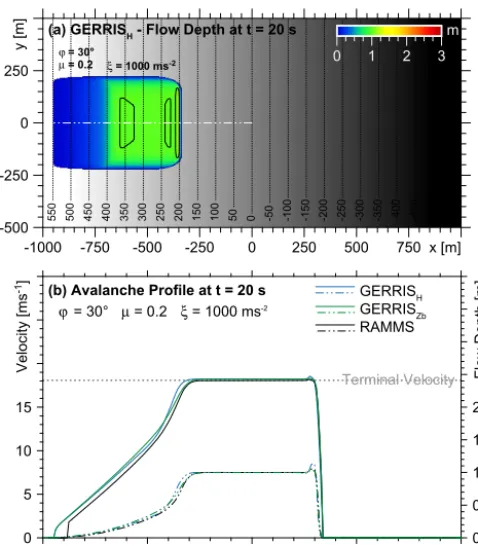
To test whether our approach reproduces this behaviour correctly, we consider a planar ramp withϕ=30◦ inclina-tion in x direction with Voellmy parameters µ=0.2 and ξ=1000 m s−2. The release zone is defined by a rectangular area of 350 m×400 m (in horizontal projection) at the upper edge of the ramp with a release height ofh=1 m measured normal to the topography. Figure 2a shows the topography and the flow depth after 20 s, obtained from the simulation with GERRISHwhere the frictional terms (i.e.ψ in Eq. 21) are computed from the surface of the flowing mass.
-550
-500
-450
-400
-350
-300
-250
-200
-150
-100
-50
0
50
100
150
200
250
300
350
400
450
500
550
(a) GERRISH - Flow Depth at t = 20 s
ϕ = 30°
µ = 0.2 ξ = 1000 ms-2
m -500
-250 0 250
y [m]
-1000 -750 -500 -250 0 250 500 750 x [m]
0 1 2 3
m
(b) Avalanche Profile at t = 20 s
ϕ = 30° µ = 0.2 ξ = 1000 ms-2
0 5 10 15
Velocity [ms
-1]
x [m] 0.0
0.5 1.0 1.5 2.0
Flow Depth [m]
GERRISH
GERRISZb
RAMMS
-500 -750
-1000 -250
Terminal Velocity
Figure 2. Comparison of two different numerical solutions of GERRIS with RAMMS for granular flow over a 30◦dipping ramp for Voellmy parametersµ=0.2 and ξ=1000 m s−2 and an ini-tial flow depthh=1 m . (a) Two-dimensional representation of the ramp geometry and the flow depth of the fluid layer measured nor-mal to the surface after 20 s. The white dashed-dotted line indicates the position of the longitudinal profiles shown in (b). (b) Longi-tudinal profiles of three different numerical models showing flow velocity (solid lines) and flow depth (dashed-dotted lines). The gray dashed line indicates the theoretical terminal velocity according to Eq. (28). GERRIS-based models (blue and green lines) apply gra-dients of fluid surface (GERRISH) and gradients of the topography (GERRISZb) respectively, and black lines are results RAMMS as reference.
numerical experiments: the realization GERRISH discussed above, the alternative approach GERRISZb where the bed surface is used to compute the friction term, and the reference model RAMMS. Only minor differences among the three models are encountered. The avalanche develops a character-istic tail with a rapidly declining flow depth in upslope direc-tion, while the initial flow depth ofh=1 m is still preserved in the main body. The avalanche has already reached the steady-state velocity of about 18 m s−1in the main body pre-dicted by Eq. (28), while the velocities in the tail are lower as a consequence of the reduced flow depth. The avalanche front of all three experiments is characterized by a slight increase of flow depth and flow velocity relative to the main avalanche body. This artefact is in general small, but most pronounced for GERRISH, while RAMMS and GERRISZbshow nearly identical profiles at the avalanche front. The slightly stronger
artefact occurring in GERRISHpresumably arises from our simple implementation of the gradient of the fluid surface re-quired for computing the anglesϕandψrequired in Eq. (24). Here we use the standard gradient of the fluid surface pro-vided by GERRIS that is computed from simple symmetri-cal difference quotients. The sophisticated numerics imple-mented in GERRIS itself used for maintaining a sharp front is not incorporated here, so that finally the driving term of the shallow water equations and the friction term use different schemes of discretization, causing artefacts at the avalanche front where the fluid surface is strongly curved. However, we found in all considered examples that these small artefacts are stable and do not grow over time, so that they are not a serious problem at all.
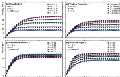
As a second test, we consider the velocity of the acceler-ating fluid layer against the time-dependent analytical solu-tion (Eq. 30) for different initial flow depths (h), turbulence (ξ) and dry friction (µ) parameters of the Voellmy rheology, and hillslope angles (ϕ) (Fig. 3). Similarly to the results on the avalanche profiles, the almost perfect agreement between the velocity predicted by Eq. (30) and all sets of numeri-cal experiments verifies the ability of our approach at least for planar slopes. Small deviations occur shortly after the re-lease scale with the time step size of the numerical model and could be reduced by forcing the flow solver towards smaller time increments. However, these initial small deviations dis-appear rapidly when approaching the terminal velocity, so that a higher temporal resolution at the expense of increasing computational time does not justify this insignificant benefit in practical applications.
4.2 The effect of profile curvature
While the tests performed in the previous section only con-cern the technical correctness of the theory and its imple-mentation, the following numerical experiments address the validity and the limitations of the approximations made.
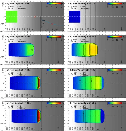
In order to explore the effects of profile curvature on our approach considering only the horizontal components of the velocity vector (and calculating the total velocity from those), we have performed a series of numerical experiments on curved synthetic topographies and compare the results of our approach with those of RAMMS. The first experiment describes an avalanche on a concave flow path defined by a 30◦ dipping ramp and a 5◦ inclined run-out zone with a smooth (parabolic) transition between both (Fig. 4). Here and in the following, the curvature of the smooth transition zone is defined in such a way that an avalanche entering from the upper ramp with the terminal velocity according to Eq. (28) is exposed to an centrifugal acceleration of about 1 m s−2 (which is neglected in both RAMMS and our approach but considered in detail by Fischer et al., 2012).
(a) Flow Depth: h
ϕ=45°
µ=0.2
ξ=1000 ms-2
h=0.5 m h=1.0 m h=2.0 m h=3.0 m h=4.0 m
0 10 20 30 40
Velocity [ms
-1] (b) Voellmy Parameter: ξ
h =1.0 m
ϕ =45°
µ =0.2
ξ=500 ms-2
ξ=1000 ms-2
ξ=1500 ms-2
ξ=2000 ms-2
ξ=2500 ms-2
(c) Voellmy Parameter: µ
h=1.0 m
ϕ=45°
ξ=1000 ms-2
µ=0.15
µ=0.20
µ=0.25
µ=0.30
µ=0.35
0 10 20
Velocity [ms
-1]
0 5 10 15 20 Time [s]
(d) Hillslope Angle:ϕ
h=1.0 m
µ=0.2
ξ=1000 ms-2
ϕ=30°
ϕ=35°
ϕ=40°
ϕ=45°
ϕ=50°
0 5 10 15 20 Time [s]
Figure 3. Test of the numerical results of GERRISZb(symbols) against the one-dimensional analytical time-dependent solution for a Voellmy fluid flowing on a flow path with a constant slope (Eq. 30, solid lines) for several parameter sets for (a) flow depthh, (b) turbulence parameter
ξ, (c) dry friction parameterµ, and (d) slope angleϕ.
mass of the avalanche remains undeformed and has reached the steady-state velocity of about 18 m s−1 (Fig. 4c, d). At this time the avalanche front approaches the curved transition zone to the gently dipping run-out zone leading to a strong deceleration and thickening. At t=60 s, the frontal part of the fluid layer is more than 3 times thicker than it initially was. The flow velocity has decreased below 10 m s−1 every-where (Fig. 4e, f). Att=80 s, the avalanche thickens further in the run-out zone and grows laterally normal to the flow path and in upslope direction as additional mass from the slower avalanche tail becomes incorporated in the deposit (fluid without significant motion). At this stage, significant flow velocities are confined to the steep flow path section where the avalanche tail is still in motion (Fig. 4g, h).
While Fig. 4 shows that the avalanche behaves as expected qualitatively, Fig. 5 provides a quantitative comparison with the reference model RAMMS. The flow depths (Fig. 5a–c) and the velocities (Fig. 5d–f) predicted by both models agree almost perfectly in the domain interesting for hazard assess-ment, i.e. where the avalanche moves at a significant velocity. The same applies to the run-out distance when the avalanche front finally comes to rest.
Noticeable differences between the results of GERRIS-based models and RAMMS only occur in the final phase of the avalanche when the front has almost come to rest. While the main body of the avalanche is characterized by a single maximum in the thickness in the GERRIS-based simulations,
RAMMS predicts a bimodal avalanche profile. This differ-ence is also reflected in the shape of the final deposits at least when the RAMMS simulation is stopped automatically using the default settings (i.e. when the momentum has decreased to 5 % of its maximum value). However, the difference arises in a phase where only the long tail of the avalanche moves at a considerable velocity, so that material is pushed from be-hind on the main avalanche body that it already almost rest-ing. So this difference is probably not related to the different way of treating velocities but rather to the different numeri-cal schemes used in RAMMS and GERRIS; apart from this, it is unimportant for practical purposes.
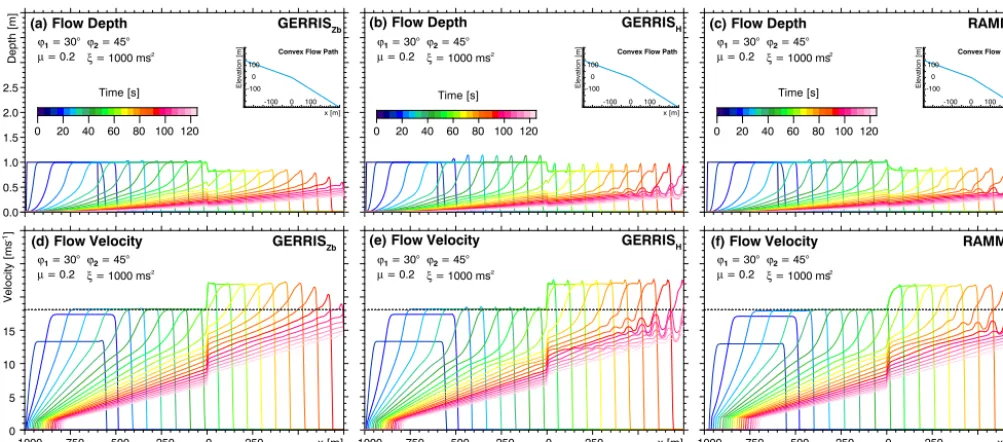
In Fig. 6, the opposite situation involving a convex topog-raphy is considered. Again the release zone is located on a 30◦steep slope, but in contrast to the previous experiment the slope steepens in a smooth transition to 45◦. The tran-sition from ϕ1=30◦ toϕ2=45◦ causes the fluid layer to accelerate rapidly from 18 m s−1to the new terminal veloc-ity of 21.7 m s−1 at a reduced flow depth of 0.83 m. As an effect of our approximation considering only the horizontal components of the velocity vector, the new terminal veloc-ity is reached slightly earlier by GERRIS than by RAMMS. This effect becomes more pronounced by sharp terrain transi-tions (Fig. 7). In this example, the fluid moves at the terminal velocity ofv∞=18 m s−1in the upper region,
0 50 100 150 200 250 300 350 400 450 500 550
(a) Flow Depth at t = 0 s
-100 -50 0 50 100 150 200 250 300 350 400 450 500 550
(b) Flow Velocity at t = 0 s
-100 -50 0 50 100 150 200 250 300 350 400 450 500 550
(c) Flow Depth at t = 40 s
-100 -50 0 50 100 150 200 250 300 350 400 450 500 550
(d) Flow Velocity at t = 40 s ϕ -100 -50 0 50 100 150 200 250 300 350 400 450 500 550
(e) Flow Depth at t = 60 s
-100 -50 0 50 100 150 200 250 300 350 400 450 500 550
(f) Flow Velocity at t = 60 s
-100 -50 0 50 100 150 200 250 300 350 400 450 500 550
(g) Flow Depth at t = 80 s
-100 -50 0 50 100 150 200 250 300 350 400 450 500 550
(h) Flow Velocity at t = 80 s
0 10 20 30
ms-1
0 1 2 3
m
0 10 20 30
ms-1
0 1 2 3
m
0 10 20 30
ms-1
0 1 2 3
m
0 10 20 30
ms-1
0 1 2 3
m
x [m]
-1000 -750 -500 -250 0 250 500
-500 -250 0 -500 -250 0 -500 -250 0 -500 -250 0 y [m] y [m] y [m] y [m] -100 0 100 0 100 -100 1
5 10 15
5 10 5 1 12 3 1 2 3 x [m]
-1000 -750 -500 -250 0 250 500
ϕ1 = 30° ϕ2 = 5°
µ = 0.2 ξ = 1000 ms-2 ϕµ1 = 30° = 0.2 ϕξ = 1000 ms2 = 5° -2
ϕ1 = 30° ϕ2 = 5°
µ = 0.2 ξ = 1000 ms-2
ϕ1 = 30° ϕ2 = 5°
µ = 0.2 ξ = 1000 ms-2 ϕµ1 = 30° = 0.2 ϕξ = 1000 ms2 = 5° -2
ϕ1 = 30° ϕ2 = 5°
µ = 0.2 ξ = 1000 ms-2
ϕ1 = 30° ϕ2 = 5°
µ = 0.2 ξ = 1000 ms-2 ϕµ1 = 30° = 0.2 ϕξ = 1000 ms2 = 5° -2
Figure 4. Two-dimensional representation of numerical solutions of GERRISZbfor flow depth and flow velocity partly concave slope at four different time steps. The fluid layer accelerates at an inclined ramp (ϕ1=30◦) and runs out in a gently dipping surface (ϕ2=5◦) with a smooth (parabolic) transition starting atx=0. A topographic profile of the geometry is shown in the inset of (a). The white dashed-dotted line indicates the position of the longitudinal profiles shown in Figs. 5 and 6.
proach, the velocity immediately after the transition amounts to v= vh
cosϕ2 =22 m s
−1, which is even slightly above the new terminal velocity. However, the avalanche of RAMMS
also reaches the terminal velocity rapidly after entering the steeper region for both the smooth and the sharp transition.
0 20 40 60 80 100 120 Time [s]
(a) Flow Depth GERRISZb
ϕ1 = 30°ϕ2 = 5°
µ = 0.2 ξ = 1000 ms-2
Concave Flow Path
-100 0 100
0 100 -100
x [m]
Elevation [m]
(f) Flow Velocity RAMMS
ϕ1 = 30°ϕ2 = 5°
µ = 0.2 ξ = 1000 ms-2
(d) Flow Velocity GERRISZb
ϕ1 = 30°ϕ2 = 5°
µ = 0.2 ξ = 1000 ms-2
0 20 40 60 80 100 120 Time [s]
(c) Flow Depth RAMMS
Concave Flow Path
-100 0 100
0 100 -100
x [m]
Elevation [m]
ϕ1 = 30°ϕ2 = 5°
µ = 0.2 ξ = 1000 ms-2
(e) Flow Velocity GERRISH
ϕ1 = 30°ϕ2 = 5°
µ = 0.2 ξ = 1000 ms-2 0 20 40 60 80 100 120
Time [s]
(b) Flow Depth GERRISH
ϕ1 = 30°ϕ2 = 5°
µ = 0.2 ξ = 1000 ms-2
Concave Flow Path
-100 0 100
0 100 -100
x [m]
Elevation [m]
0.0 0.5 1.0 1.5 2.0 2.5
Depth [m]
0 5 10 15
Velocity [ms
-1]
-1000 -750 -500 -250 0 250 x [m] -1000 -750 -500 -250 0 250 x [m] -1000 -750 -500 -250 0 250 x [m]
Figure 5. Time series of longitudinal profiles plotted every 5 s for flow depth and flow velocity of the scenario shown in Fig. 4. Profiles are based on numerical solutions of (a, d) GERRISZb(b, e) GERRISH, and (c, f) RAMMS. The insets show the topographic profile.
0 20 40 60 80 100 120
Time [s]
(a) Flow Depth GERRISZb
0.0 0.5 1.0 1.5 2.0 2.5
Depth [m]
Convex Flow Path
-100 0 100
0 100 -100
x [m]
Elevation [m]
ϕ1 = 30°ϕ2 = 45°
µ = 0.2 ξ = 1000 ms-2
0 20 40 60 80 100 120
Time [s]
(c) Flow Depth RAMMS
Convex Flow Path
-100 0 100
0 100 -100
x [m]
Elevation [m]
ϕ1 = 30°ϕ2 = 45°
µ = 0.2 ξ = 1000 ms-2
0 20 40 60 80 100 120 Time [s]
(b) Flow Depth GERRISH
ϕ1 = 30°ϕ2 = 45°
µ = 0.2 ξ = 1000 ms-2
Convex Flow Path
-100 0 100
0 100 -100
x [m]
Elevation [m]
(d) Flow Velocity GERRISZb
0 5 10 15
Velocity [ms
-1]
ϕ1 = 30°ϕ2 = 45°
µ = 0.2 ξ = 1000 ms-2
-1000 -750 -500 -250 0 250 x [m]
(e) Flow Velocity GERRISH
ϕ1 = 30°ϕ2 = 45°
µ = 0.2 ξ = 1000 ms-2
-1000 -750 -500 -250 0 250 x [m]
(f) Flow Velocity RAMMS
ϕ1 = 30°ϕ2 = 45°
µ = 0.2 ξ = 1000 ms-2
-1000 -750 -500 -250 0 250 x [m]
Figure 6. Time series of longitudinal profiles plotted every 5 s for flow depth and flow velocity of a granular fluid on a convex slope with
ϕ=30◦,ϕ=45◦, and a smooth transition between the two segments. Profiles are obtained from numerical solutions of (a, d) GERRISZb, (b, e) GERRISH, and (c, f) RAMMS. The insets show the topographic profile.
can be derived from the theoretical considerations made in Sect. 4.1. Instead of the velocity as a function of time, we now consider the velocity as a function of the travelled dis-tance. Using Eq. (29) we obtain
dv
dx =
dv
dt
dx
dt
=
g ξ h v
2
∞−v2
v (32)
≈ 2g
ξ h(v∞−v) for v≈v∞. (33)
Equation (33) implies thatvapproaches the terminal velocity v∞exponentially with decay length
L=ξ h
2g. (34)
constant influx instead of a constant flow depth, i.e. hv=
const, leads to basically the same result where only the factor 2 in the denominator turns into a factor 3. Thus, the avalanche should practically approach the terminal velocity even more rapidly than stated above.
Returning to Fig. 6, the only significant difference between the results of the two GERRIS-based models and RAMMS occur at a late stage (t >80 s) where the direct effect of our approximation should have almost vanished. As the avalanche becomes more and more stretched at the backward side, the region with a constant thickness becomes shorter until it finally vanishes. In the simulation with GERRISZb, this leads to a rapid decrease in flow depth and consequently in velocity, so that the avalanche decays rapidly. In contrast, RAMMS keeps a sharper distinction between the region of constant flow depth and consequently maintains the original flow depth and velocity for a longer time. In return, rather strong waves occur at the transition to the tail being visible in both flow depth and flow velocity. Such waves are in prin-ciple generated by GERRISZb, too, but with a significantly smaller amplitude than in RAMMS. In return, GERRISH generates even stronger oscillations than RAMMS.
Similarly to the differences among the models found for the concave topography, the differences found here are pre-sumably not related to our approximation of considering only the horizontal velocity and computing the total velocity after-wards but rather to the different discretization schemes used in RAMMS and GERRIS. GERRIS itself obviously uses a numerical scheme that is well suited for reducing oscilla-tions at the transition to the avalanche tail, but our simple implementation of the gradient of the fluid surface used in GERRISHcannot compete with this scheme.
In summary, the numerical experiments with GERRIS and the comparison with the leading avalanche model RAMMS performed in this section demonstrate the ability of our ap-proach to model avalanches even on curved topography. The effects of our approximations cause only minor deviations, and in particular their impact on predictions of run-out dis-tance, flow depth, and velocity is practically negligible. The better stability of both the avalanche front and the transition to the tail provides arguments in favour of GERRISZb com-pared to GERRISH.
4.3 Flow over complex topography
The thalweg of rapid mass movements on a real topography is in general curved and twisted. We therefore challenge our approach with the complex topography of a typical alpine avalanche flow path and test the results of our approach against RAMMS. In contrast to the previous examples that are in their basic structure one-dimensional, the second ap-proximation made in our theory also becomes relevant here: beyond considering only the horizontal component of the ve-locity in the equations, our approach only applies corrections
for large slopes to the longitudinal component of the acceler-ation.
The hypothetical avalanche is located in the Felbertal, a typical glacially shaped alpine valley with large open flanks between ridges and the tree line representing classic snow avalanche release zones. Deeply incised, curved and twisted gullies canalize the avalanche in one or several branches with locally extreme flow depths. These gullies route the granular fluid to the nearly flat valley floor, representing the run-out zone of the avalanche (Fig. 8).
We compare the maximum values (at each point, taken over the entire simulation) of flow depth, momentum, and velocity of the modelled avalanche. We set the release height toh=1 m and define spatially constant parameters for the Voellmy flow resistance law (µ=0.2,ξ=2000 m s−2). All simulations are performed on a quadrilateral grid with a spa-tial resolution of 4 m and terminate when the momentum of the fluid drops below 5 % of the maximum momentum (de-fault of RAMMS).
Generally, the deviations among GERRISZb, GERRISH, and RAMMS are small, and the primary features of the avalanche agree well between the two GERRIS approaches and RAMMS. This includes flow depths, run-out distances, flow velocities, and momentum.
However, a closer examination reveals some deviations be-tween the different numerical approaches. RAMMS shows a more pronounced tendency to overflow counter hillsides and to keep the flow direction even uphill. This is clearly documented at the lower third of the avalanche track where the avalanche is split into two branches. Here the orographic right flow path is characterized by a considerable uphill sec-tion. In this domain, the results of RAMMS show higher values in the maximum flow depth compared to the two GERRIS approaches (Fig. 8a–c). The modelled avalanches in RAMMS overflow larger areas, causing a wider flow path than predicted by the GERRIS experiments. This is recognized most clearly in the s-shaped gully section. The broader flow path and tendency to flow uphill, observed in avalanches modelled with RAMMS relative to those mod-elled with GERRISZb and GERRISH, are caused by larger values in the momentum (Fig. 8d–f) arising from slightly higher flow velocities especially in the gully section of the thalweg (Fig. 8g–i).
0 20 40 60 80 100 120 Time [s]
(a) Flow Depth GERRISZb
ϕ1 = 30°ϕ2 = 45°
µ = 0.2 ξ = 1000 ms-2
Depth [m]
0.0 0.5 1.0 1.5 2.0 2.5
Convex Flow Path
-100 0 100
0 100 -100
x [m]
Elevation [m]
(d) Flow Velocity GERRISZb
0 5 10 15
Velocity [ms
-1]
ϕ1 = 30°ϕ2 = 45°
µ = 0.2 ξ = 1000 ms-2
-1000 -750 -500 -250 0 250 x [m]
0 20 40 60 80 100 120 Time [s]
(c) Flow Depth RAMMS
ϕ1 = 30°ϕ2 = 45°
µ = 0.2 ξ = 1000 ms-2 Convex Flow Path
-100 0 100
0 100 -100
x [m]
Elevation [m]
(f) Flow Velocity RAMMS
ϕ1 = 30°ϕ2 = 45°
µ = 0.2 ξ = 1000 ms-2
-1000 -750 -500 -250 0 250 x [m]
(e) Flow Velocity GERRISH
ϕ1 = 30°ϕ2 = 45°
µ = 0.2 ξ = 1000 ms-2
(b) Flow Depth GERRISH
-1000 -750 -500 -250 0 250 x [m]
0 20 40 60 80 100 120 Time [s]
Convex Flow Path
-100 0 100
0 100 -100
x [m]
Elevation [m]
ϕ1 = 30°ϕ2 = 45°
µ = 0.2 ξ = 1000 ms-2
Figure 7. Time series of longitudinal profiles plotted for the scenario considered in Figs. 6 and 7 but with a sharp transition between the planar slope segments.
A further deviation is observed in the run-out zone where the shapes of the avalanche deposit of the RAMMS simu-lations differ considerably from those of the GERRIS sim-ulations, while the run-out distances and base areas of the avalanche deposits of the three models agree well. The dis-crepancy in the geometry of the deposits is similar to that found when considering the run-out on the simple concave topography in Sect. 4.2, and it is presumably related to the different numerical schemes used in RAMMS and GERRIS rather than to our approximations.
Finally, the differences between the realizations GERRISH, where the corrections in the friction term are based on the fluid surface, and GERRISZb, where the corrections are computed from the original topography, are very small in this example. So the stronger (although not serious) artefacts occurring at the avalanche front in GERRISH(Sect. 4.1) and the higher stability of GERRISZb at the transition to the tail remain the only noticeable difference between both GERRIS-based approaches. These differences suggest that using the version GERRISZbmay in general be preferable to GERRISH.
5 Conclusions
The examples considered in Sect. 4 show that granular avalanches can be simulated using the shallow water equa-tions directly in Cartesian coordinates even in steep terrain when an appropriate additional friction term is included. This finding allows the utilization of software that was originally designed for other purposes, namely modelling the flow of water in rivers, lakes, and oceans.
Compared to software packages explicitly developed for modelling avalanches, a wealth of state-of-the-art fluid dy-namics software packages potentially being adjustable for this purpose is available. Some of them are even freely avail-able. Therefore, research on avalanches can easily profit from the enormous effort that has already been spent in develop-ing numerical codes in fluid dynamics. The implementations presented in this paper are based on the software GERRIS, but this should only be seen as an example. Apart from be-ing freely available and providbe-ing state-of-the-art numerics, GERRIS allows the implementation of our method with a moderate effort. However, this should not imply that GER-RIS is the best software for this purpose.
386000 387000 388000 389000 386000 387000 388000 389000
(b) Flow Depth GERRISH
0 2 4 6 8 10 m
h = 1 m µ = 0.2 ξ = 2000 ms-2
(h) Flow Velocity GERRISH
0 10 20 30 40 50 ms-1 h = 1 m µ = 0.2 ξ = 2000 ms-2
232000 233000 234000
(d) Momentum GERRISZb
0 100 200 300 m2s-1 h = 1 m µ = 0.2 ξ = 2000 ms-2
(c) Flow Depth RAMMS
0 2 4 6 8 10 m
h = 1 m µ = 0.2 ξ = 2000 ms-2
232000 233000 234000
(a) Flow Depth GERRISZb
0 2 4 6 8 10 m
h = 1 m µ = 0.2 ξ = 2000 ms-2
(i) Flow Velocity RAMMS
0 10 20 30 40 50 ms-1 h = 1 m µ = 0.2 ξ = 2000 ms-2
232000 233000 234000
386000 387000 388000 389000
(g) Flow Velocity GERRISZb
0 10 20 30 40 50 ms-1 h = 1 m µ = 0.2 ξ = 2000 ms-2
(f) Momentum RAMMS
0 100 200 300 m2s-1 h = 1 m µ = 0.2 ξ = 2000 ms-2
(e) Momentum GERRISH
0 100 200 300 m2s-1 h = 1 m µ = 0.2 ξ = 2000 ms-2
Figure 8. Maximum values of the characteristic properties of a hypothetical avalanche flowing along a curved and twisted thalweg on a real topography (Felbertal, Austria), based on the numerical solutions of GERRISZb, GERRISH, and RAMMS for the same model set-up. Fluid rheology (µ=0.2,ξ=2000 m s−2) and spatial resolution for the three different numerical models are the same. (a–c) maximum flow depth, (d–f) maximum momentum, (g–i) maximum flow velocity.
The example based on a complex topography (Sect. 4.3) reveals still rather small, but perhaps not always negligible, differences between our approach and RAMMS. RAMMS solutions show larger flow depths in avalanche tracks with prominent uphill sections and expanded overflowed areas in steep, twisted gullies. In contrast to the differences discussed above, these deviations arise from the approximations dis-cussed in Sect. 3 and represent a small intrinsic model limita-tion that is inevitable when using the shallow water equalimita-tion in a Cartesian coordinate system with a friction term acting only in direction opposite to the velocity.
However, when discussing differences between models on such a small level we should keep in mind that all these mod-elling approaches involve a considerable inherent uncertainty compared to other flow processes such as the flow of water in lakes and oceans. These uncertainties start with the basic assumption of the granular medium as a single layer con-tinuum and the rheology (e.g. Voellmy’s friction law). They continue with the determination of the relevant parameters for dry snow avalanches and do not stop at the determination
of the release zone in the form of spatial position, extent, and involved volumes (fracture depth). Even the resolution and quality of the applied digital elevation model can highly in-fluence the avalanche path (Bühler et al., 2011), and taking into account further processes such as entrainment introduces an additional uncertainty in the parameters. Assessing these uncertainties quantitatively goes beyond the scope of this pa-per, but, in summary, they are obviously larger than the small deviations between the models.
The differences between the two proposed implemen-tations based on GERRIS are also small. The version GERRISZb where the correction terms are computed from the original topography is less prone to artefacts at the avalanche front and at the transition to the tail than the ver-sion GERRISHusing the fluid surface, without revealing sig-nificant drawbacks anywhere. We therefore suggest comput-ing the friction terms from the topographic slope instead of the fluid surface.
rapid mass movements such as debris flows. Debris flows are characterized by lower flow velocities and lower flow path gradients compared to snow avalanches, so that effects of our approximations become even less significant. Besides model set-ups with a pre-defined release volume, a huge number of scenarios involving different release zones characterized by discharge time series can be easily implemented within the GERRIS parameter file. In principle the initiation of surface runoff can be defined at each mesh element, so that flooding and debris flow simulations based on precipitation time series for storm events are possible without preceding precipitation runoff models. Flow resistance laws and their parameteriza-tions are also defined in the parameter file, so that the imple-mentation of other rheological models (e.g. Bingham fluid) is straightforward and requires no specific coding skills.
Appendix A: Implementation in GERRIS
The following lines of code show the implementation of our approach in the GERRIS parameter file. An example of a full implementation (the concave slope considered in Sect. 4.2) is provided in the supplement.
# Gradient of the original topography (GERRISZb) # For version GERRISHreplaceZbwithH
#Variables:P=hv, (U,V)=q
DX=dx("Zb") DY=dy("Zb") #tan2ϕ(Eq. 7)
TAN2PHI=DX·DX+DY·DY
#sin2ϕfrom basic trigonometric relations
SIN2PHI=TAN2PHI/(1.+TAN2PHI)
#cosϕfrom basic trigonometric relations
COSPHI=1./sqrt(1+TAN2PHI)
#tanψ(Eq. 8), directions ofqandvhare the same
TANPSI=-(DX·U+DY·V)/sqrt(U·U+V·V+eps) #cosψfrom basic trigonometric relations
COSPSI=1./SQRT(1+TANPSI·TANPSI)
#Factor 1+1δtf occurring in Eq. (24) withf from Eq. (20)
F=(P > DRY ? Velocity/(Velocity ...
+dt·GRAV·(SIN2PHI·TANPSI ...
+mu·COSPHI·COSPSI+Velocity·Velocity ...
/(P·Xi·COSPHI·COSPSI))) : 0. )
#Multiply both components of the momentum byF (Eq. 24)
U=U·F V=V·F
#Magnitude of the three-dimensional velocity vector
Vtotal=(P > DRY ? Velocity/COSPSI : 0)
#Flow depth normal to the topography
Acknowledgements. We thank ILF Consulting Engineers for licensing RAMMS in the course of a common project and the federal government of Salzburg for implementing the INSPIRE guidelines and providing ALS digital elevation models with a resolution of 10 m. Furthermore, we thank T. Glade for the editorial handling and P. Bartelt for comments on the software RAMMS during the discussion phase and acknowledge the willingness of two anonymous reviewers to provide comments on this study. We acknowledge financial support by the Open Access Publication Fund of the University of Salzburg.
Edited by: T. Glade
Reviewed by: two anonymous referees
References
An, H. and Yu, S.: Well-balanced shallow water flow simula-tion on quadtree cut cell grids, Adv. Water Resour., 39, 60–70, doi:10.1016/j.advwatres.2012.01.003, 2012.
Berger, M. J., George, D. L., LeVeque, R. J., and Man-dli, K. T.: The GeoClaw software for depth-averaged flows with adaptive refinement, Adv. Water Resour., 34, 1195–1206, doi:10.1016/j.advwatres.2011.02.016, 2011.
Bouchut, F. and Westdickenberg, M.: Gravity driven shallow water models for arbitrary topography, Commun. Math. Sci., 2, 359– 389, 2004.
Bühler, Y., Christen, M., Kowalski, J., and Bartelt, P.: Sen-sitivity of snow avalanche simulations to digital elevation model quality and resolution, Ann. Glaciol., 52, 72–80, doi:10.3189/172756411797252121, 2011.
Christen, M., Kowalski, J., and Bartelt, P.: RAMMS: Nu-merical simulation of dense snow avalanches in three-dimensional terrain, Cold Reg. Sci. Technol., 63, 1–14, doi:10.1016/j.coldregions.2010.04.005, 2010.
Fischer, J.-T., Kowalski, J., and Pudasaini, S. P.: Topographic cur-vature effects in applied avalanche modeling, Cold Reg. Sci. Technol., 74–75, 21–30, doi:10.1016/j.coldregions.2012.01.005, 2012.
Granig, M. and Jörg, P.: A dynamic aproach to evaluate the dense and powder snow avalanche model SAMOS-AT, in: 12th Congress Interpraevent, 23–26 April 2012, Grenoble, France, Extended Abstracts, edited by: Koboltschnig, G., Hübl, J., and Braun, J., 196–197, 2012.
Horton, P., Jaboyedoff, M., Rudaz, B., and Zimmermann, M.: Flow-R, a model for susceptibility mapping of debris flows and other gravitational hazards at a regional scale, Nat. Hazards Earth Syst. Sci., 13, 869–885, doi:10.5194/nhess-13-869-2013, 2013. Hsu, S. M., Chiou, L. B., Lin, G. F., Chao, C. H., Wen, H. Y., and
Ku, C. Y.: Applications of simulation technique on debris-flow hazard zone delineation: a case study in Hualien County, Taiwan, Nat. Hazards Earth Syst. Sci., 10, 535–545, doi:10.5194/nhess-10-535-2010, 2010.
Keiler, M., Sailer, R., Jörg, P., Weber, C., Fuchs, S., Zischg, A., and Sauermoser, S.: Avalanche risk assessment – a multi-temporal approach, results from Galtür, Austria, Nat. Hazards Earth Syst. Sci., 6, 637–651, doi:10.5194/nhess-6-637-2006, 2006.
Kirschbaum, D. B., Adler, R., Hong, Y., Hill, S., and Lerner-Lam, A.: A global landslide catalog for hazard applications: Method, results, and limitations, Nat. Hazards, 52, 561–575, doi:10.1007/s11069-009-9401-4, 2010.
LeVeque, R. J., George, D. L., and Berger, M. J.: Adaptive Mesh Refinement Techniques for Tsunamis and Other Geo-physical Flows Over Topography, Acta Numer., 20, 211–289, doi:10.1017/S0962492911000043, 2011.
Medina, V., Hürlimann, M., and Bateman, A.: Application of FLAT-Model, a 2D finite volume code, to debris flows in the north-eastern part of the Iberian Peninsula, Landslides, 5, 127–142, doi:10.1007/s10346-007-0102-3, 2008.
Mergili, M., Schratz, K., Ostermann, A., and Fellin, W. C.: Physically-based modelling of granular flows with Open Source GIS, Nat. Hazards Earth Syst. Sci., 12, 187–200, doi:10.5194/nhess-12-187-2012, 2012.
Popinet, S.: An accurate adaptive solver for surface-tension-driven interfacial flows, J. Comput. Phys., 228, 5838–5866, doi:10.1016/j.jcp.2009.04.042, 2009.
Popinet, S.: Adaptive modelling of long-distance wave propaga-tion and fine-scale flooding during the Tohoku tsunami, Nat. Hazards Earth Syst. Sci., 12, 1213–1227, doi:10.5194/nhess-12-1213-2012, 2012.
Pudasaini, S. P. and Hutter, K.: Rapid shear flows of dry granular masses down curved and twisted channels, J. Fluid Mech., 495, 193–208, doi:10.1017/S0022112003006141, 2003.
Pudasaini, S. P. and Hutter, K.: Avalanche Dynamics – Dynamics of Rapid Flows of Dense Granular Avalanches, Springer, Berlin, Heidelberg, New York, 215–223, 2007.
Pudasaini, S. P., Wang, Y., and Hutter, K.: Modelling debris flows down general channels, Nat. Hazards Earth Syst. Sci., 5, 799– 819, doi:10.5194/nhess-5-799-2005, 2005.
Pudasaini, S. P., Sheng, L.-T., Hsiau, S.-S., Hutter, K., and Katzen-bach, R.: Avalanching granular flows down curved and twisted channels: theoretical and experimental results, Phys. Fluids, 20, 073202, doi:10.1063/1.2945304, 2008.
Sailer, R., Fellin, W., Fromm, R., Jörg, P., Rammer, L., Sampl, P., and Schaffhauser, A.: Snow avalanche mass-balance calculation and simulation-model verification, Ann. Glaciol., 48, 183–192, doi:10.3189/172756408784700707, 2008.
Sampl, P. and Zwinger, T.: Avalanche simulation with SAMOS, Ann. Glaciol., 38, 393–398, doi:10.3189/172756404781814780, 2004.
Sheridan, M. F., Stinton, A. J., Patra, A., Pitman, E. B., Bauer, A., and Nichita, C. C.: Evaluating Titan2D mass-flow model using the 1963 Little Tahoma Peak avalanches, Mount Rainier, Washington, J. Volcanol. Geotherm. Res., 139, 89–102, doi:10.1016/j.jvolgeores.2004.06.011, 2005.
Voellmy, A.: Über die Zerstörungskraft von Lawinen, Schweiz. Bauzeitung, 73, 159–165, 212–217, 246–249, 280–285, 1955. Vreugdenhil, C. B.: Numerical Methods for Shallow-Water Flow,
Springer, Berlin, Heidelberg, New York, 262 pp., 1994. Weller, H. and Weller, H. G.: A high-order arbitrarily